
Technical publication
Back to publications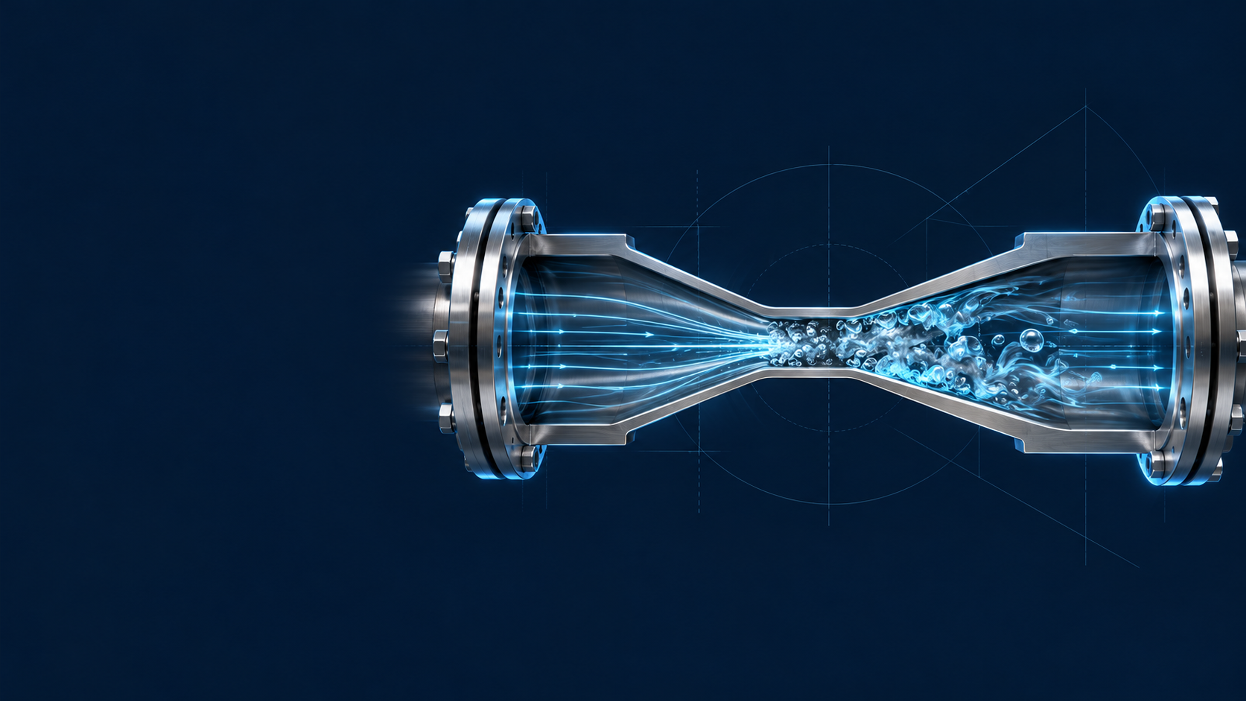
Reactors & equipment
Calculations of Hydrodynamic Cavitation Devices
okozyuk.com
Published
Read complete publication for whole-document Find and printing. Browser Find and native printing on this reader include only loaded content.
7 Integrated Design, Scale Up, and Commissioning Procedure
The calculation of a cavitation device should culminate in an integrated operating envelope rather than a single design point. Flow, inlet pressure, backpressure, temperature, speed, gas content, viscosity, solids loading, and number of passes interact. The acceptable operating region is the intersection of cavitation performance, product response, power, temperature, mechanical integrity, cleanability, and material loss constraints.
7.1 Calculation sequence
A complete design sequence is as follows:
Define the process objective. State the required transformation and quantitative acceptance variables, including distributions rather than only averages where relevant.
Define the feed envelope. Tabulate density, viscosity or rheology, vapor pressure, gas condition, solids, surface tension, corrosive species, and temperature at minimum, normal, and maximum conditions.
Define the system boundary. Identify whether power is hydraulic, shaft, or electrical; whether energy is reported per pass, per batch, per unit mass, or per product output; and whether the pump is included.
Select the cavitation mechanism. Choose a restriction, Venturi, wake, multistage arrangement, vortex chamber, or dynamic rotor according to flow, passage size, control range, cleanability, and maintenance.
Complete the preliminary hydraulic calculation. Determine areas, velocities, , , , pressure profile, , residence time, power, and expected recovery location.
Complete the mechanical screen. Calculate pressure boundary demand, rotor stress where applicable, clearance, torque, supports, thermal growth, and pressure cycle or speed cycle requirements.
Allocate materials by function. Separate pressure boundary, wear insert, collapse liner, rotor, stator, seal, and product contact requirements.
Calibrate the equipment coefficients. Measure , recovery coefficient, , , and other geometry specific quantities on the actual or a rigorously similar unit.
Map cavitation and process response. Vary pressure drop or speed, flow, backpressure, temperature, gas, and passes. Record both hydraulic state and product response.
Validate the uncertain model. Use CFD, visualization, dynamic pressure, acoustic data, tracer tests, or wear coupons according to the unresolved design question.
Run an endurance test. Confirm power, temperature, vibration, erosion, corrosion, fouling, cleanability, and product contamination.
Freeze the operating envelope and inspection interval. Define controls, alarms, dimensional limits, spare parts, and recalibration after wear or maintenance.
7.2 Operating map
A useful operating map contains, at minimum, flow on one axis and pressure drop or rotational speed on the other. Contours or labels identify:
-
no or weak cavitation;
-
inception and intermittent cavities;
-
developed useful operating region;
-
connected or supercavitating region where collapse may be displaced;
-
excessive temperature rise;
-
power or torque limit;
-
vibration or noise limit;
-
product quality acceptance region;
-
erosion or contamination limit.
The optimum operating condition is application specific. The largest visible vapor cloud does not necessarily correspond to maximum reaction rate, breakup, disinfection, or energy efficiency. A stable connected cavity can reduce the number of discrete collapse events, whereas excessive backpressure can suppress useful cavity growth. The operating map should therefore be defined by the measured process objective [2–10].
7.3 Heat balance
Most mechanical and hydraulic energy eventually appears as heat unless it leaves as pressure energy, shaft work, chemical free energy, phase change, acoustic radiation, or kinetic energy. The approximate adiabatic temperature rise over a treatment is:
where is mass specific energy converted to internal energy and is specific heat capacity. For water, 1 kJ/kg corresponds to approximately 0.24 K if all energy becomes sensible heat. In a recirculation loop, cumulative temperature rise changes vapor pressure and viscosity and can move the device into a different cavitation regime. Temperature must therefore be controlled or incorporated into the operating map.
For a steady cooled loop, the required heat removal rate is approximately:
where represents desired enthalpy carried by product and represents other energy leaving the boundary. In most nonthermal applications, the cooling duty is close to net electrical input after external motor and drive losses are accounted for.
7.4 Pump and system matching for static devices
The operating point of a pump driven cavitator is the intersection of the pump curve and system curve. For a system with static head and approximately quadratic losses,
where includes the cavitator, piping, valves, heat exchanger, and fittings at the stated fluid properties. A variable frequency drive changes the pump curve and can provide flow control, but reducing speed also changes available pressure. A downstream control valve can set backpressure, yet it must not become an uncontrolled cavitation source.
The pump suction calculation should use the lowest liquid level, highest temperature, greatest suction line loss, and maximum gas condition. The process device is intended to cavitate; the pump inlet is not. Pump cavitation changes flow, pressure, vibration, and power and invalidates the device calculation.
7.5 Acceptance calculations
The design acceptance report should reconcile measured and calculated quantities. A normalized deviation is:
for each quantity , such as flow, pressure drop, shaft power, electrical power, temperature rise, or product response. Acceptance limits should reflect measurement uncertainty and model purpose. A 3% flow deviation may be important for a narrow multihole operating point, while a larger deviation may be acceptable in an early concept screen.
Table 7.1. Integrated calculation and commissioning record.
| Topic | Calculated or specified value | Measured value | Uncertainty | Acceptance criterion | Status |
|---|---|---|---|---|---|
| Flow rate and turndown | |||||
| Inlet and outlet absolute pressure | |||||
| Pressure drop or rotor speed | |||||
| Minimum pressure or inception indicator | |||||
| Hydraulic, shaft, and electrical power | |||||
| Specific energy | |||||
| Temperature rise and cooling duty | |||||
| Product quality attributes | |||||
| Vibration or acoustic signature | |||||
| Dimensional wear and metal release | |||||
| Cleaning and drainability |
7.6 Summary of worked calculations
Table 7.2. Comparison of the four examples worked.
| Device | Primary design variable | Calculated operating result | Principal calibration need |
|---|---|---|---|
| Eight hole orifice | Total open area from , , and | Eight 3.81 mm holes; 15.21 m/s nominal jet; 0.417 kW hydraulic power | Actual , vena contracta pressure, jet interaction and erosion |
| Venturi | Throat area from target minimum pressure | 10.86 mm ideal throat at 10 m³/h; diffuser length 0.092 to 0.280 m for 12° to 4° | Two phase throat pressure, diffuser recovery and cavity length |
| Vortex chamber | Circulation and finite core radius | m²/s for the selected radii and pressure | Relation between inlet momentum and circulation; vapor core model |
| Rotor stator | Tip speed and calibrated power number | 28.35 m/s; 5.50 kW; 18.4 N·m; 570 Hz passage frequency | , local pressure, clearance effects, vapor fraction and endurance |