Calculations of Hydrodynamic Cavitation Devices

Abstract

Hydrodynamic cavitation devices generate controlled vapor and gas vapor cavities by imposing a local pressure depression followed by pressure recovery. Reliable design therefore requires more than a single cavitation threshold or dimensionless index. This article presents a calculation framework for static, vortex, and dynamic hydrodynamic cavitation devices and integrates hydraulic sizing, pressure reference selection, dimensionless analysis, energy input, residence time, cavity collapse, uncertainty, mechanical integrity, materials selection, scale translation, and commissioning. Static device calculations address orifices, nozzles, slits, Venturi passages, bluff bodies, and multistage arrangements. Vortex device calculations combine tangential inlet sizing with radial equilibrium screening and finite core limitations. Dynamic device calculations include rotor tip speed, rotational Reynolds number, cavitation number, power number, torque, rotor stator clearance, feature passage frequency, stress, vibration, and thermal growth. Worked examples demonstrate preliminary sizing for an eight hole orifice plate, an ideal Venturi throat, a finite core vortex chamber, and a rotor stator operating point. The analysis emphasizes that local pressure history, cavity structure, process response, and erosion cannot be inferred reliably from global pressure drop alone. Calibrated coefficients, validated computational fluid dynamics, representative pilot testing, and measured operating maps are required to establish a defensible design envelope and service life.

1 Introduction

Hydrodynamic cavitation occurs when the pressure history experienced by a flowing liquid permits preexisting nuclei to expand into vapor filled or gas vapor cavities and subsequently subjects those cavities to sufficiently rapid pressure recovery. In static devices, this pressure history is produced by acceleration through a fixed restriction, flow separation, jet expansion, wake formation, or swirl. In dynamic devices, rotors, rotor stator clearances, pin arrays, cavities, grooves, or moving blades repeatedly create regions of reduced pressure followed by recovery. Although the governing physical principles are common, calculation procedures cannot be transferred directly among device families [1–7].

Three recurring design errors should be avoided. First, cavitation should not be treated as a binary condition. A local pressure below vapor pressure indicates the potential for vapor formation, but it does not define cavity population, cloud structure, residence time, collapse intensity, process response, or erosion rate. Second, the measured upstream to downstream pressure difference should not be interpreted as the local minimum pressure. A wall tap averages pressure over a finite region and may not detect conditions at a vena contracta, separated shear layer, vortex core, rotor cavity, or transient blade passage. Third, no single dimensionless group constitutes a complete scale up criterion. Reynolds number, Euler number, Weber number, cavitation number, flow coefficient, power number, and residence time each preserve only part of the coupled system behavior [3–12].

A defensible design calculation is therefore organized into four levels. The first level is a transparent one dimensional or lumped parameter screening model that establishes required flow area, mean velocity, pressure drop, power, nominal residence time, pressure boundary load, and a preliminary cavitation regime. The second level applies calibrated discharge, loss, recovery, power, or circulation coefficients obtained from water testing or a geometrically similar device. The third level uses validated computational fluid dynamics when local pressure, vapor fraction, recirculation, or rotor stator interaction cannot be represented adequately by a lumped model. The fourth level is pilot confirmation in the actual process fluid because viscosity, vapor pressure, dissolved gas, suspended solids, non Newtonian behavior, interfacial tension, reaction kinetics, and contamination limits can shift the useful operating window [5, 7, 10–15].

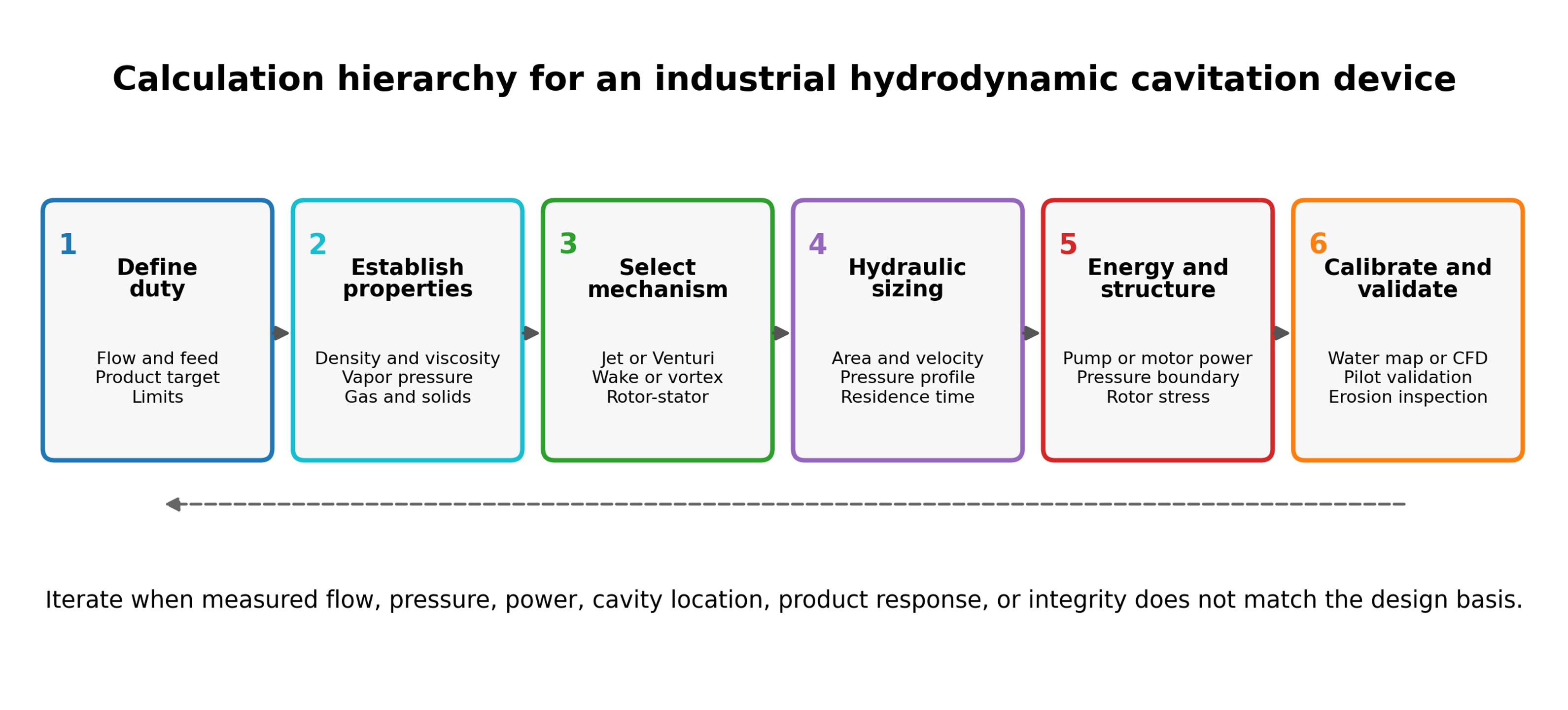
Figure 1.1. Calculation hierarchy for an industrial hydrodynamic cavitation device [32].

The objective of the calculation is not to predict every individual bubble. It is to establish a traceable design basis and identify the assumptions that require calibration or experimental confirmation. The calculation record should answer the following questions:

• What flow rate and feed property envelope must be processed?

• Which absolute pressure is expected at the active cavitation location?

• Where will cavities grow, and where should they collapse?

• What pump or motor power is required at the selected operating point?

• What exposure, residence time, number of stages, or number of passes is delivered?

• Which part is the pressure boundary, which part is a wear insert, and which parts must be hygienic or chemically inert?

• How will the hydraulic state, product response, erosion, contamination, and uncertainty be verified?

This article uses SI units unless stated otherwise. All pressures used in vapor pressure and cavitation number calculations are absolute. Gauge pressure is used only after explicit conversion. Correlations should not be transferred between geometries without a stated technical basis, and calculated values should be reported with sufficient significant figures for reproducibility without implying unrealistic precision.

2 Calculation Basis and Design Workflow

This section defines the consolidated calculation and reporting framework used throughout the article. Subsequent sections apply consistent definitions for absolute pressure, cavitation number, hydraulic and electrical energy, residence time, exposure, uncertainty, and scale translation. Equations are repeated only when a specialized derivation or interpretation is required.

2.1 Required design inputs

The calculation begins with the process duty rather than a preferred device configuration. The minimum data set in Table 2.1 separates properties required for hydraulic sizing from variables required for process validation and mechanical design. A single nominal density and viscosity are insufficient when temperature, composition, gas content, or solids loading varies during operation.

Table 2.1. Minimum design inputs for hydrodynamic cavitation calculations.

Category	Required information	Calculation affected
Capacity	Minimum, normal, and maximum volumetric or mass flow; batch and loop volume; required turndown	Flow area, velocity, pump or motor size, residence time, parallel modules
Pressure	Suction pressure, upstream pressure, downstream pressure, backpressure, allowable pressure drop, relief set pressure	Local pressure screen, cavitation number, pressure boundary, pump duty
Temperature	Minimum, normal, and maximum temperature; allowable temperature rise	Density, viscosity, vapor pressure, seal compatibility, thermal growth
Liquid properties	Density, dynamic viscosity, vapor pressure, speed of sound, surface tension where relevant	Reynolds number, cavitation inception, collapse, pressure transients
Multiphase properties	Gas content, gas solubility, solids loading and size, dispersed phase fraction, rheology	Nucleation, blockage, wear, phase separation, model selection
Product objective	Reaction conversion, droplet or particle distribution, cell disruption, contaminant removal, heating, gas dispersion	Required exposure, passes, energy, sampling and acceptance limits
Geometry constraints	Pipe size, available length, cleanability, minimum passage, allowable rotor diameter and clearance	Device family, throat or hole size, diffuser length, rotor layout
Materials environment	pH, chloride, oxidants, solvents, acids, caustic, abrasive solids, hygiene requirements	Alloy, coating, elastomer, corrosion allowance, surface finish
Utilities	Electrical supply, pump curve, cooling duty, nitrogen or gas injection, instrumentation	Installed power, control strategy, heat exchanger and interlocks
Reliability	Inspection interval, permitted metal contamination, spare strategy, acceptable downtime	Replaceable inserts, erosion allowance, monitoring and lifecycle cost

Material properties should be evaluated at each relevant operating state. For water like liquids, vapor pressure changes rapidly with temperature and can dominate the cavitation margin. For viscous oils, concentrated suspensions, polymer solutions, and emulsions, apparent viscosity may be shear dependent and pressure losses outside the cavitation element may no longer be negligible. The design envelope should therefore include startup, shutdown, cleaning, upset, and maximum temperature conditions rather than only the nominal process state.

2.2 Pressure references and measurement stations

Pressure must be placed on an absolute basis before it is compared with vapor pressure:

where $p_{abs}$ is absolute pressure, $p_g$ is gauge pressure, and $p_{atm}$ is local atmospheric pressure. A vacuum gauge reading requires the corresponding sign convention. Barometric variation is usually small relative to a high pressure device, but it can be important in low pressure systems and suction calculations.

The instrumentation arrangement should establish reproducible pressure stations upstream and downstream of the cavitation element while recognizing that these taps do not normally measure the local minimum pressure. Rapid pressure pulsation may require high frequency transducers in addition to conventional process transmitters. Tap diameter, distance from the element, pipe diameter, straight length, tubing volume, transducer range, and sampling frequency should be documented [2,4–6].

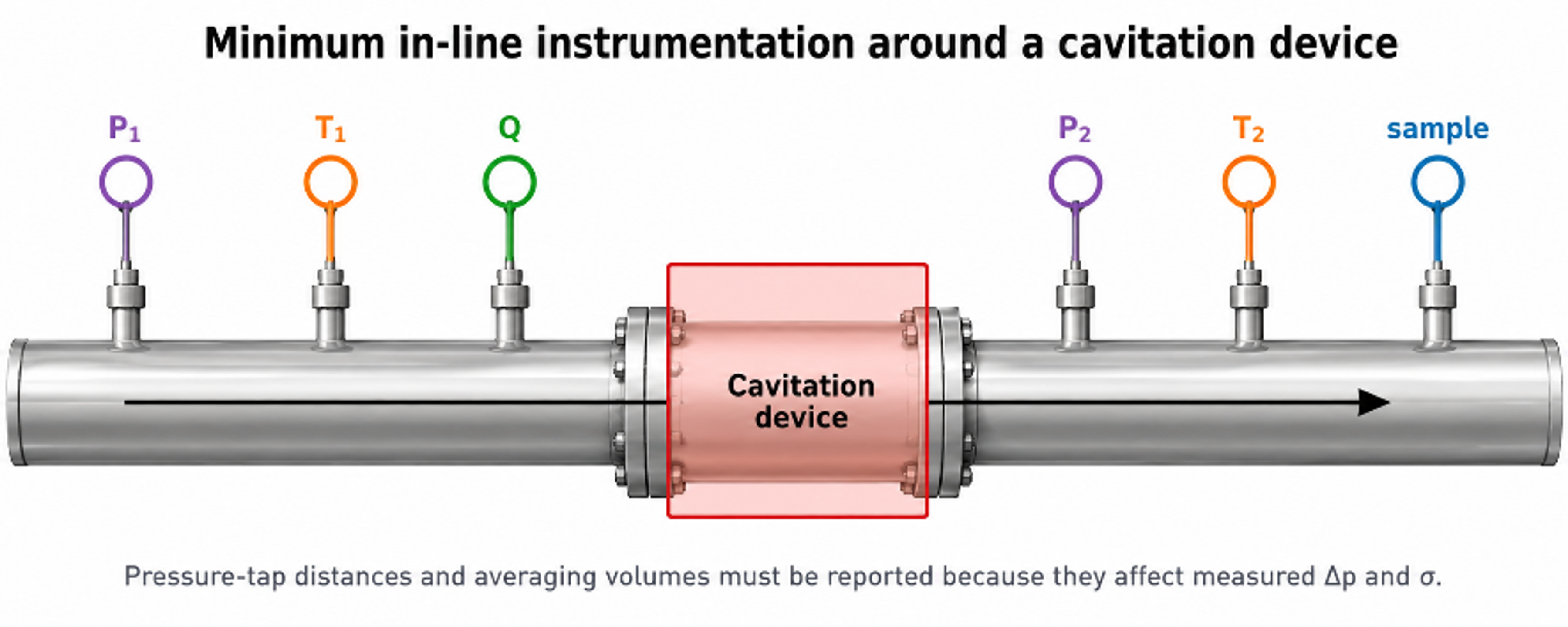
Figure 2.1. Minimum instrumentation around the flow through cavitation element [32].

For an incompressible stream, volumetric flow and mass flow are:

where $Q$ is volumetric flow rate, $A$ is cross sectional area, $\bar{V}$ is mean velocity, $\dot{m}$ is mass flow rate, and $\rho$ is density.

A practical mechanical energy balance between stations 1 and 2 is:

where $g$ is gravitational acceleration, $z$ is elevation, $h_p$ is head added by a pump within the control volume, $h_L$ is irreversible head loss, and $\alpha$ is the kinetic energy correction factor. For a short horizontal element with no pump between the taps, the elevation and pump terms are omitted. The equation remains an averaged energy balance; it does not resolve the local pressure depression inside a separated, swirling, or transient flow.

Figure 2.2 illustrates the importance of local pressure history. A sharp restriction may generate a short, steep pressure minimum followed by highly dissipative recovery, whereas a well designed Venturi can provide a longer low pressure region with more controlled recovery. These conceptual profiles do not replace calibrated pressure measurements, but they inform throat length, diffuser geometry, and the placement of downstream surfaces.

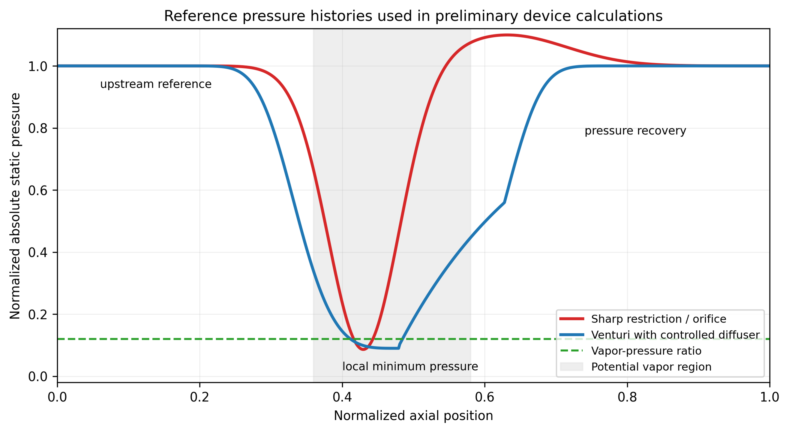
Figure 2.2. Conceptual absolute pressure histories for a sharp restriction and a Venturi with controlled recovery [32].

2.3 Dimensionless groups

The Reynolds number based on a stated characteristic length $D_c$ and velocity $V_c$ is:

where $\mu$ is dynamic viscosity. The Euler number, written here as a pressure loss coefficient, is

The Weber number is:

where $\gamma$ is surface or interfacial tension. For two phase dispersions, the relevant interfacial tension and characteristic droplet or jet dimension must be specified.

The general cavitation number is:

where $p_{ref}$ and $V_{ref}$ are explicitly defined reference pressure and velocity, and $p_v$ is vapor pressure at the local temperature. Published values are not comparable unless the reference stations and velocity definition are the same. For an orifice study, $p_{ref}$ may be downstream pressure and $V_{ref}$ the jet velocity; for a Venturi it may be throat or downstream pressure and throat velocity; for a rotor it may be chamber pressure and rotor tip speed [2–6].

A pressure drop cavitation index frequently used in flow through equipment is:

where $p_1$ and $p_2$ are stated upstream and downstream absolute pressures. This form is convenient because the denominator is measured pressure drop, but it still does not resolve the local minimum pressure. It should be treated as an operating index tied to the test geometry.

The preliminary vapor formation criterion is:

and a preliminary collapse criterion is:

where $p_{\min }$ is the calculated or modeled local minimum pressure and $p_{rec}$ is the pressure in the intended recovery region. Inception can occur above equilibrium vapor pressure because of gas nuclei and unsteady pressure, while a cavity can persist after the mean pressure has recovered. Equations (2.10) and (2.11) are therefore screening conditions rather than exact phase boundary laws [1–3].

Table 2.2. Interpretation and limitations of principal similarity groups.

Group	Principal comparison	Must be defined	Important limitation
$Re$	Inertia relative to viscosity	Velocity and length scale	Does not preserve nuclei, vapor fraction, collapse location, or residence time
$Eu$	Pressure change relative to dynamic pressure	Pressure stations and velocity	Can global pressure loss match while local pressure fields differ
$We$	Inertia relative to surface or interfacial tension	Interface and length scale	Relevant to breakup, but not sufficient for recoalescence or chemistry
$\sigma$	Pressure margin above vapor pressure	Absolute pressure and velocity reference	Definition varies by device; one value cannot describe a full pressure history
$C_v$	Downstream pressure margin normalized by measured loss	Upstream and downstream taps	Does not directly measure vena contracta, core, or blade passage pressure
$St$	Unsteady frequency relative to convection	Characteristic frequency and length	Frequency similarity does not guarantee the same vapor cloud amplitude
$Po$	Shaft power is relative to rotational inertial scale	Shaft power, speed, rotor diameter	Geometry, clearance, flow coefficient, and gas fraction must remain comparable

2.4 Hydraulic power, electrical power, residence time, and dose

The hydraulic power associated with a measured pressure drop is:

For a pump driven static device, the approximate electrical input assigned to the cavitation duty is:

where ${\eta }_p$ is pump efficiency, ${\eta }_m$ is motor efficiency, and ${\eta }_d$ represents drive or transmission efficiency. For a complete system assessment, auxiliary loads, recirculation losses, cooling, and control equipment should be included. Measured electrical power is preferred over nameplate power.

The single pass hydraulic specific energy is:

and the corresponding mass specific electrical energy over a treatment interval $t$ is:

A short device volume $V_d$ has nominal residence time:

For a well mixed recirculation tank of volume $V_L$, the nominal number of loop turnovers during time $t$ is:

This turnover count does not guarantee that each fluid element has passed through the device exactly $N_{turn}$ times. A real loop has a residence time distribution, short circuiting, dead volume, and mixing effects. For comparison of process results, the report should include the tank volume, external piping volume, device hold up, flow history, sample location, and whether the product is withdrawn continuously or only after recirculation [2–5].

2.5 Collapse time and placement of the recovery zone

A useful inertial estimate for the collapse time of an initially spherical vapor cavity of radius $R_0$ under a constant pressure difference is the Rayleigh expression:

where $p_{\infty }$ is the recovered far field pressure. The corresponding convective distance is:

where $V_c$ is a representative convection velocity. These equations do not include dissolved gas, thermal effects, non spherical collapse, cloud interaction, or wall proximity, but they help place a replaceable collapse chamber, avoid a vulnerable weld, and estimate whether a long low pressure zone will carry cavities beyond the intended active region [1,2].

For example, a water vapor cavity with $R_0=0.5$ mm exposed to a recovered pressure difference of 200 kPa has an inertial collapse time of approximately 32 microseconds. At a convection velocity of 12 m/s, the corresponding distance is approximately 0.38 mm. Real clouds can persist much farther because of gas content, collective shielding, repeated growth, and spatially distributed pressure recovery. The calculation is therefore a lower order location screen, not an erosion life prediction.

2.6 Uncertainty and model hierarchy

For a result $y=f(x_1,x_2,\dots ,x_n)$ with independent input uncertainties, the first order combined standard uncertainty is:

where $u_{x_i}$ is the standard uncertainty of input $x_i$. Correlated variables require covariance terms. A design calculation should separate measurement uncertainty from model form uncertainty. The latter includes uncertainty in discharge coefficient, pressure recovery coefficient, vortex core model, power number, two phase closure, and the relationship between hydraulic state and product response.

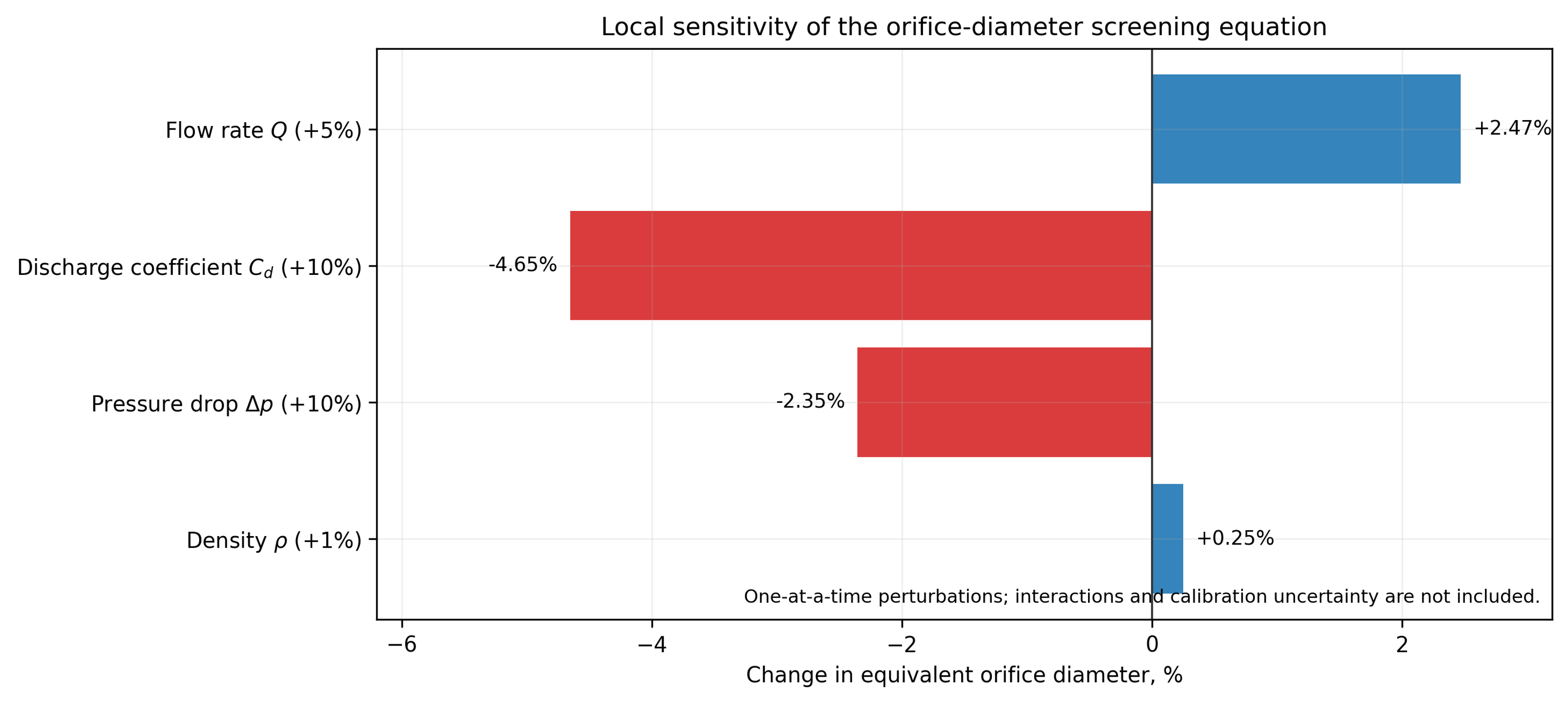
Figure 2.3. Local sensitivity of the preliminary orifice diameter equation to representative input perturbations. The result illustrates parameter sensitivity and does not include model form or interaction uncertainty [32].

Table 2.3. Recommended model fidelity by design question.

Design question	Minimum method	Escalation trigger	Validation evidence
Required open area and pump pressure	One dimensional continuity and calibrated loss coefficient	Non Newtonian flow, gas fraction, severe choking, uncertain $C_d$	Flow pressure curve at operating temperature
Local cavitation inception	Pressure screen plus calibrated inception map	Geometry has separation, vortex core, multiple jets, or transient rotor interaction	Visualization, acoustic signature, high speed pressure, or validated CFD
Cavity extent and collapse location	Empirical map or two phase CFD	Erosion sensitive surface, reaction selectivity, scale change	Imaging, erosion coupons, hydrophone or pressure mapping
Rotor power	Calibrated $Po$, torque measurement, motor map	Clearance, flow coefficient, gas fraction, or rheology changes	Shaft torque and electrical power over full operating map
Product performance	Empirical response surface	Composition, temperature, or scale differs from test	Replicated pilot trials and product analysis
Erosion life	Comparative material tests and pilot inserts	Long service interval, toxic metal limit, corrosive abrasive fluid	Periodic mass/thickness loss and contaminant analysis

The dominant uncertainty is often not the pressure measurement itself but the assumption that a hydraulic index predicts the required process response. A pilot program should therefore map hydraulic variables and product attributes concurrently. A model should be accepted only within the region where measured flow, pressure, power, temperature, cavity signature, process response, and equipment integrity remain mutually consistent.

3 Calculations for Static Hydrodynamic Cavitation Devices

Static hydrodynamic cavitation devices contain no moving cavitation generating element. Pump pressure energy is converted into local kinetic energy, separated flow, vortex motion, and irreversible pressure recovery. Principal calculation families include fixed restrictions such as orifices, nozzles, slit plates, and perforated inserts; Venturi and converging diverging passages; bluff bodies and jet impingement elements; and multistage combinations. Vortex chambers are mechanically static but are treated separately in Section 4 because their calculation method is distinct.

Static devices offer simple pressure containment, eliminate rotating seals, permit replaceable inserts, and integrate directly into pipelines. Their limitations include pump power demand, possible clogging, sensitivity to edge condition and fouling, and the possibility that attached cavities collapse near a wall. Static sizing should therefore determine both nominal hydraulic resistance and the intended locations of pressure depression and recovery [2–6].

3.1 Flow through orifice, nozzle, and slit devices

An orifice device divides the flow among one or more apertures. A sharp edged opening produces a contracted jet downstream of the physical aperture, and the minimum pressure commonly occurs near the vena contracta rather than at the downstream pressure tap. A rounded nozzle reduces separation and can shift inception and recovery. A slit provides a high perimeter to area ratio and can form a sheet like cavitation region, but it may be more sensitive to deformation, solids, and edge wear. Multi hole plates distribute flow among multiple jets and can increase the number of active regions; however, jet interaction, ligament thickness, plate thickness, and downstream chamber diameter become integral design variables [2,4–6].

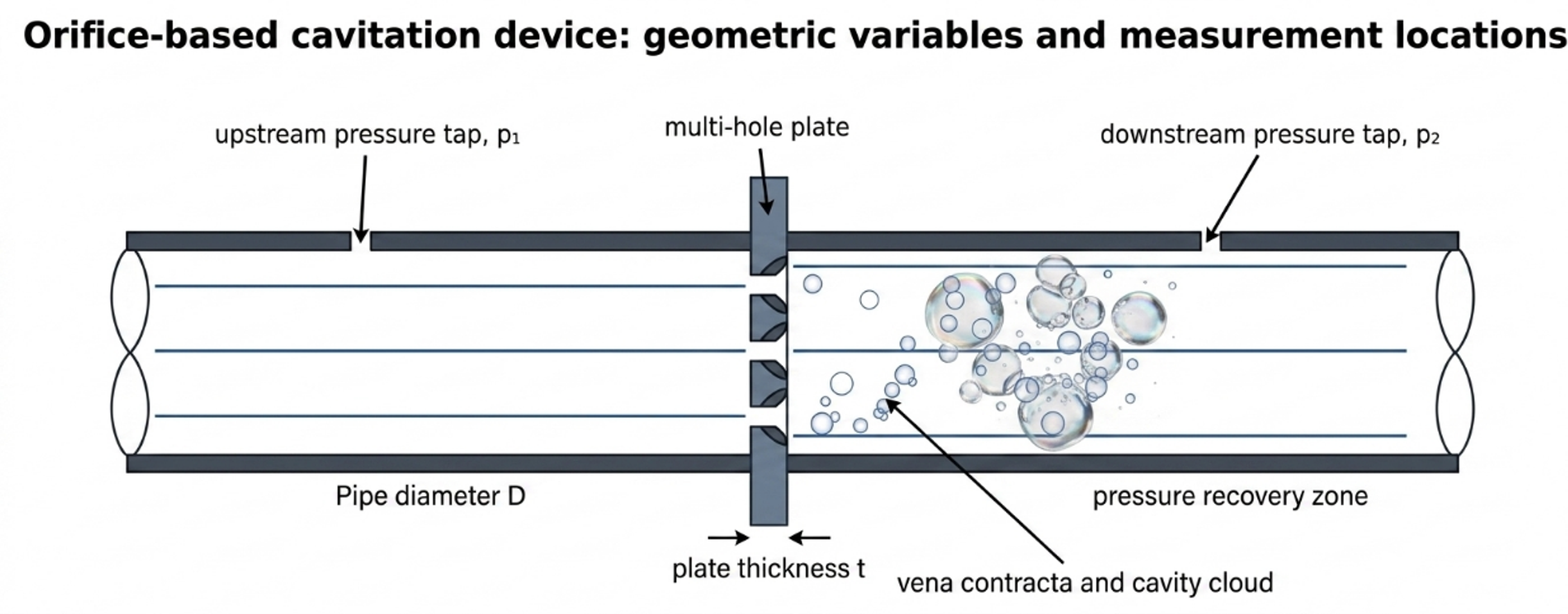
Figure 3.1. Flow through orifice geometry, principal dimensions, and pressure stations [32].

For an incompressible liquid, the basic calibrated relation is:

where $C_d$ is the discharge coefficient, $A_o$ is total open area, and $\mathrm{\Delta }p$ is the pressure difference associated with the stated measurement stations. Rearrangement gives the required total area:

For $N_h$ equal circular holes,

where $d_h$ is individual hole diameter. The nominal mean jet velocity based on the physical open area is:

and the hole Reynolds number is:

Two geometric ratios should be reported. The total open area fraction is:

where $A_p$ is pipe cross sectional area. The equivalent diameter ratio is:

where $D_p$ is pipe diameter and $d_{eq}$ is the diameter of one circular opening having the same total area. For a multi hole plate, ${\beta }_{eq}$ does not describe hole spacing, jet interaction, or minimum ligament. The individual ratio $d_h/D_p$ should also be reported.

The vena contracta area can be written $A_{vc}=C_c{A}_o$, where $C_c$ is the contraction coefficient. A one dimensional pressure screen is:

where $\mathrm{\Delta }{p}_{irr,1\to vc}$ represents irreversible loss accumulated before the vena contracta. Both $C_c$ and the local loss are geometry dependent. Equation (3.8) is useful for identifying whether the selected pressure drop can plausibly reach vapor pressure, but the result should not be presented as a measured minimum pressure unless it has been calibrated.

The pressure loss corresponding to the calibrated orifice relation is:

This quadratic dependence means that flow redistribution, fouling, edge damage, or partial blockage can change pressure drop sharply. A differential pressure alarm is therefore useful for both process control and condition monitoring.

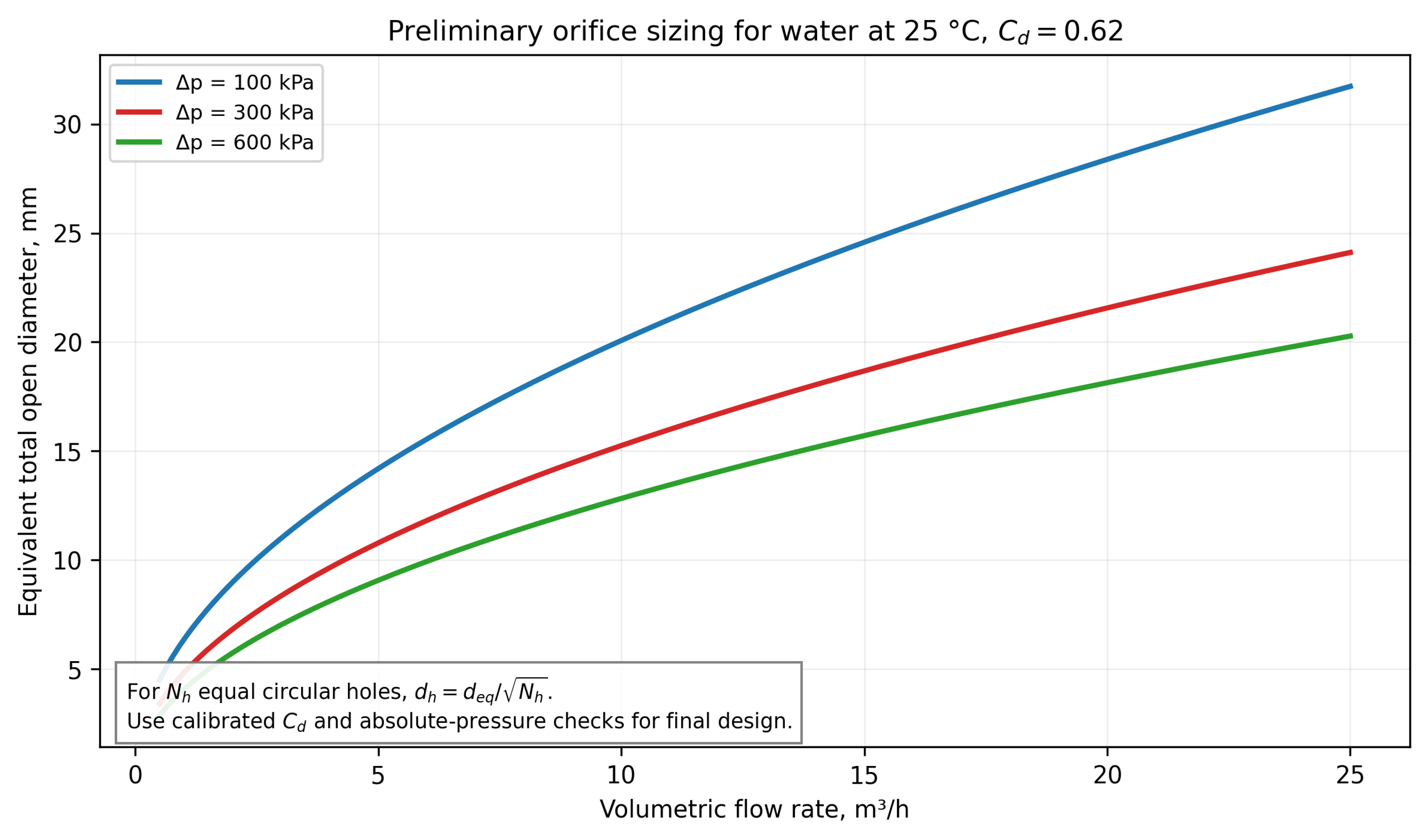
Figure 3.2. Equivalent total open diameter versus water flow for three pressure drops using a preliminary discharge coefficient C_d = 0.62 [32].

Selection and calibration of the discharge coefficient

The discharge coefficient is not a material constant. It represents contraction and energy loss and depends on Reynolds number, plate thickness to hole ratio, inlet edge radius, chamfer, hole shape, surface roughness, interaction among multiple holes, upstream velocity profile, and pressure tap arrangement. Standard differential pressure flow meter correlations such as ISO 5167 provide useful references for specified metering geometries, but a cavitating process insert may operate outside their validated geometry and flow regime [15, 16]. The recommended procedure is:

• Calculate a preliminary area using a conservative coefficient range.

• Fabricate a replaceable insert with measured dimensions and edge finish.

• Obtain a non cavitating water flow pressure curve over the intended Reynolds number range.

• Fit $C_d$ or a direct loss correlation using the exact pressure stations.

• Increase temperature or reduce backpressure to map cavitation inception and developed regimes.

• Repeat in the process fluid and check for viscosity, gas, solids, and rheology effects.

A pressure flow fit is more useful than a single coefficient because it reveals regime changes. If $C_d$ inferred from Equation (3.1) changes abruptly, the cause may be two phase choking, gas release, flow redistribution among holes, measurement dynamics, or a transition in the cavity structure.

Hole pattern and mechanical limits

A multi hole calculation must include more than total open area. Minimum hole diameter should be checked against the largest credible solid, fiber, agglomerate, crystal, or cleaning debris. The plate should retain adequate ligament between adjacent holes and between each hole and the outer sealing diameter. Plate bending, differential pressure, thermal shock, fatigue, and stress concentration around openings must be evaluated according to the applicable pressure code and fabrication standard. A thin sharp edge can produce a repeatable separated jet but is more susceptible to erosion and deformation; a thicker insert is mechanically stronger but alters the jet and may behave as a short tube.

For sanitary service, holes and downstream chambers must be inspectable and cleanable. A nominally self cleaning high velocity opening can still retain fibrous solids, crystallized salts, gums, or product in a low velocity recess. Hydraulic design should therefore be coordinated with drainability, clean in place velocity, gasket intrusion, and provision for a bypass or removable cartridge.

Table 3.1. Variables required to define a flow through restriction.

Variable	Symbol or description	Design significance
Pipe and chamber diameter	$D_p$, $D_c$	Upstream velocity, expansion ratio, recovery, jet interaction
Number and shape of openings	$N_h$; circular, slit, annular, conical	Distribution of jets, perimeter, blockage and cleanability
Opening dimension	$d_h$, slit width and length	Velocity, Reynolds number, minimum particle clearance
Total open area	$A_0$	Primary flow pressure sizing variable
Plate or insert thickness	$t_p$	Short tube behavior, strength, erosion path
Edge radius or chamfer	$r_e$ and angle	Separation and contraction coefficient
Hole pitch and ligament	$s_h$, $l_g$	Jet interaction, plate stress, manufacturability
Downstream standoff	$L_s$	Collapse location relative to wall, baffle, or next stage
Pressure tap locations	$L_{p1}$, $L_{p2}$	Reproducibility of $\mathrm{\Delta }p$, $C_d$, and $C_v$
Surface finish and material	roughness, alloy, coating	Inception, fouling, erosion, contamination

Worked Example 3.1: eight hole orifice plate

Design basis. Water at 25 °C is processed at $Q=5.00$ m³/h through a 40 mm internal diameter pipe. The selected measured pressure drop is 300 kPa. A preliminary discharge coefficient of 0.62 is used for sizing. The downstream reference pressure is absolute 150 kPa. Eight equal circular holes are selected. Water properties are $\rho =997$ kg/m³, $\mu =0.00089$ Pa·s, and $p_v=3.17$ kPa absolute.

Equation (3.2) gives:

$$A_o=9.13\times {10}^{-5}{m}^2$$

The equivalent single opening is 10.78 mm in diameter. Equation (3.3) gives an individual hole diameter of 3.81 mm. The nominal jet velocity from Equation (3.4) is 15.21 m/s, and Equation (3.5) gives $R{e}_o=6.50\times {10}^4$. The pipe area is $1.257\times {10}^{-3}$ m², so the total open area fraction is 0.0727. The ratio of each hole diameter to pipe diameter is 0.0953; the equivalent total diameter ratio is 0.2695.

The hydraulic power from Equation (2.12) is 416.7 W. If the aggregate pump, motor, and drive efficiency is 0.65, the assigned electrical input from Equation (2.13) is approximately 641 W. The single hydraulic energy pass from Equation (2.14) is 300.9 J/kg, equivalent to 0.0836 kWh per metric ton. Using downstream pressure and nominal jet velocity in Equation (2.8) gives $\sigma =1.27$. This value is only a defined operating index; the vena contracta pressure may be much lower than the downstream tap pressure.

Table 3.2. Worked Example 3.1 results.

Quantity	Value	Design interpretation
Flow rate	5.00 m³/h	Normal operating point; turndown and maximum flow also require checks
Measured pressure drop	300 kPa	Determines pump duty and calibrated flow relation
Total open area	91.3 mm²	Preliminary value using $C_d=0.62$
Number of holes	8	Must be coordinated with pitch and ligament
Individual hole diameter	3.81 mm	Verify solids clearance, tolerance, and erosion allowance
Nominal jet velocity	15.21 m/s	Physical area velocity, not vena contracta velocity
Hole Reynolds number	$6.50\times {10}^4$	Turbulent screening condition
Total open area fraction	7.27%	Strong contraction and downstream expansion
Hydraulic power	0.417 kW	Power transferred across the measured pressure drop
Estimated electrical power	0.641 kW	Uses aggregate efficiency 0.65; verify by measured input
Single pass hydraulic energy	300.9 J/kg	Does not specify the fraction delivered as useful collapse energy
Defined cavitation number	1.27	Based on $p_2=150$ kPa absolute and $V_j$; not directly comparable to other definitions

This example is a preliminary hydraulic size, not a final plate drawing. Final design requires the flow pressure curve, absolute inlet and outlet pressures, hole tolerance, edge profile, plate stress, gasket and flange details, pressure relief, minimum passage, and a cavitation map. The example also illustrates why a device can have modest total power yet a severe local pressure history

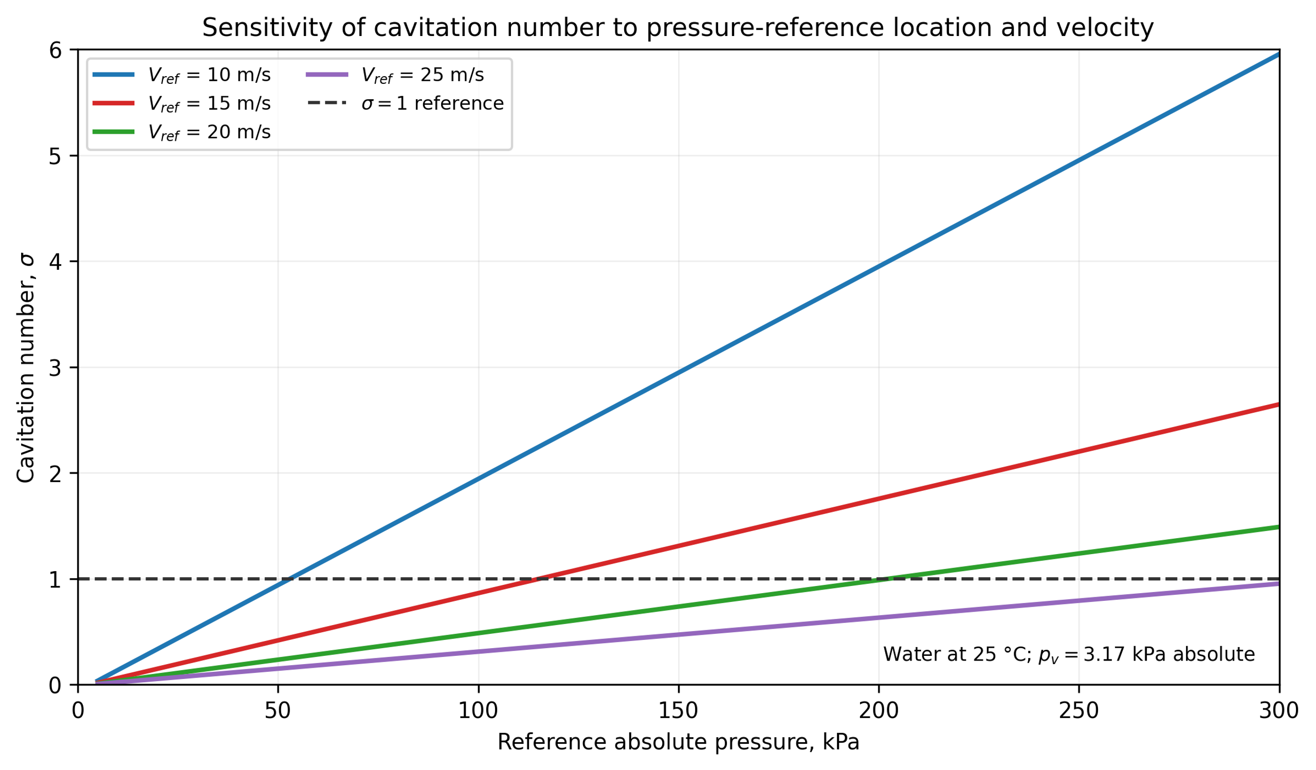
Figure 3.3. Sensitivity of the cavitation number to the selected absolute pressure and reference velocity for water at 25 °C [32].

3.2 Venturi based flow through devices

A Venturi cavitator consists of a converging section, a throat, and a diffuser. The calculation must define the contraction profile, throat diameter or hydraulic diameter, throat length, diffuser half angle, outlet diameter, surface finish, and pressure tap locations. Relative to a sharp orifice, a Venturi can provide a controlled low pressure residence interval and smoother recovery, although an aggressive diffuser can separate and generate an unsteady recovery field [4,6].

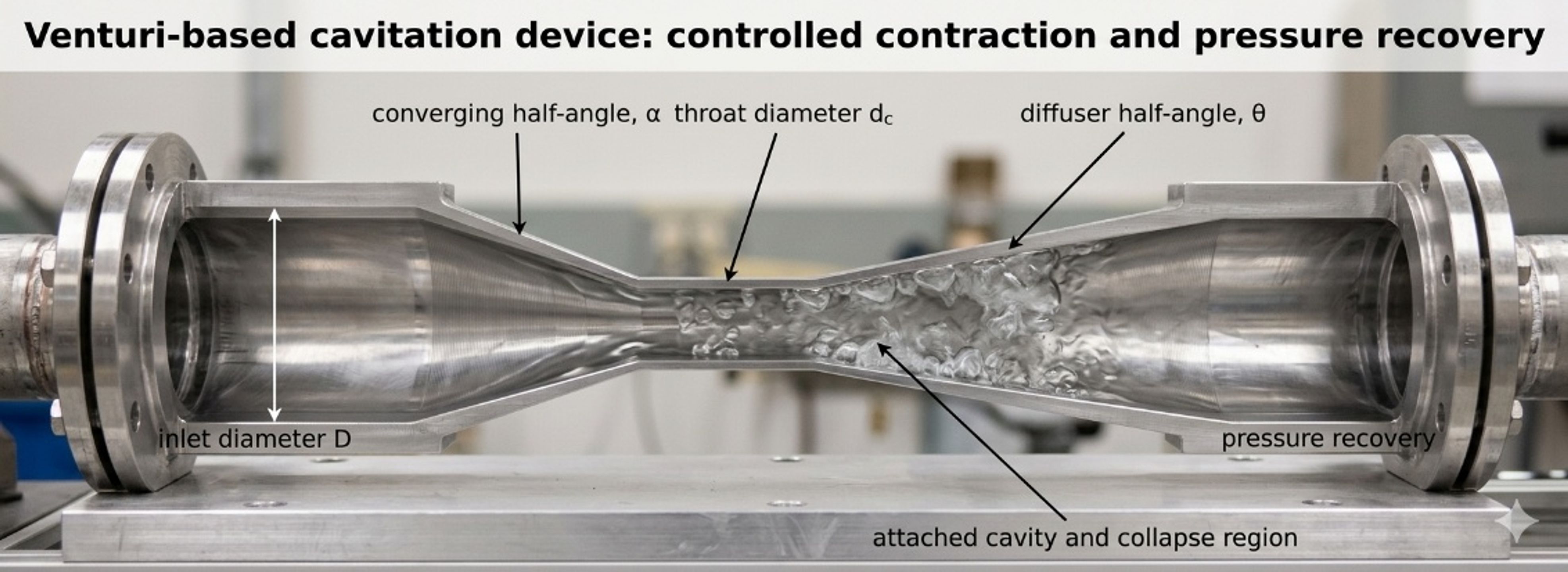
Figure 3.4. Venturi based cavitation element and principal geometric variables [32].

If the desired throat velocity is known, throat area is:

A loss free Bernoulli screen for the throat velocity is:

where $p_t$ is the selected throat pressure, usually near but not necessarily below $p_v$. This equation neglects contraction loss, wall friction, turbulence, vapor volume, and two phase choking. It therefore provides an ideal upper velocity or minimum area screen.

For a circular throat,

and the diameter ratio is:

For a calibrated incompressible Venturi relation,

where $\mathrm{\Delta }p$ is defined between the upstream and throat stations. The coefficient and tap arrangement must correspond to the actual geometry. Standard metering correlations should not be extrapolated automatically into developed cavitation or nonstandard diffuser geometries [15, 16].

Pressure recovery can be characterized by:

where $p_2$ is the downstream recovered pressure. A larger value indicates greater static pressure recovery for the defined stations, but the coefficient does not reveal local oscillation, separation, or erosion.

For a conical diffuser with half angle $\theta$,

where $D_2$ is the downstream diameter. Small angles require longer equipment but generally support more gradual recovery. Larger angles shorten the device but can increase separation. The optimum is geometry and Reynolds number dependent; final selection should use validated CFD or a measured recovery map [4,6].

For a noncircular throat, the hydraulic diameter is:

where $P_w$ is wetted perimeter. A slit Venturi may be sized using $D_h$ for Reynolds number and friction screens, but local corner flow, aspect ratio, and sidewall effects still require explicit treatment.

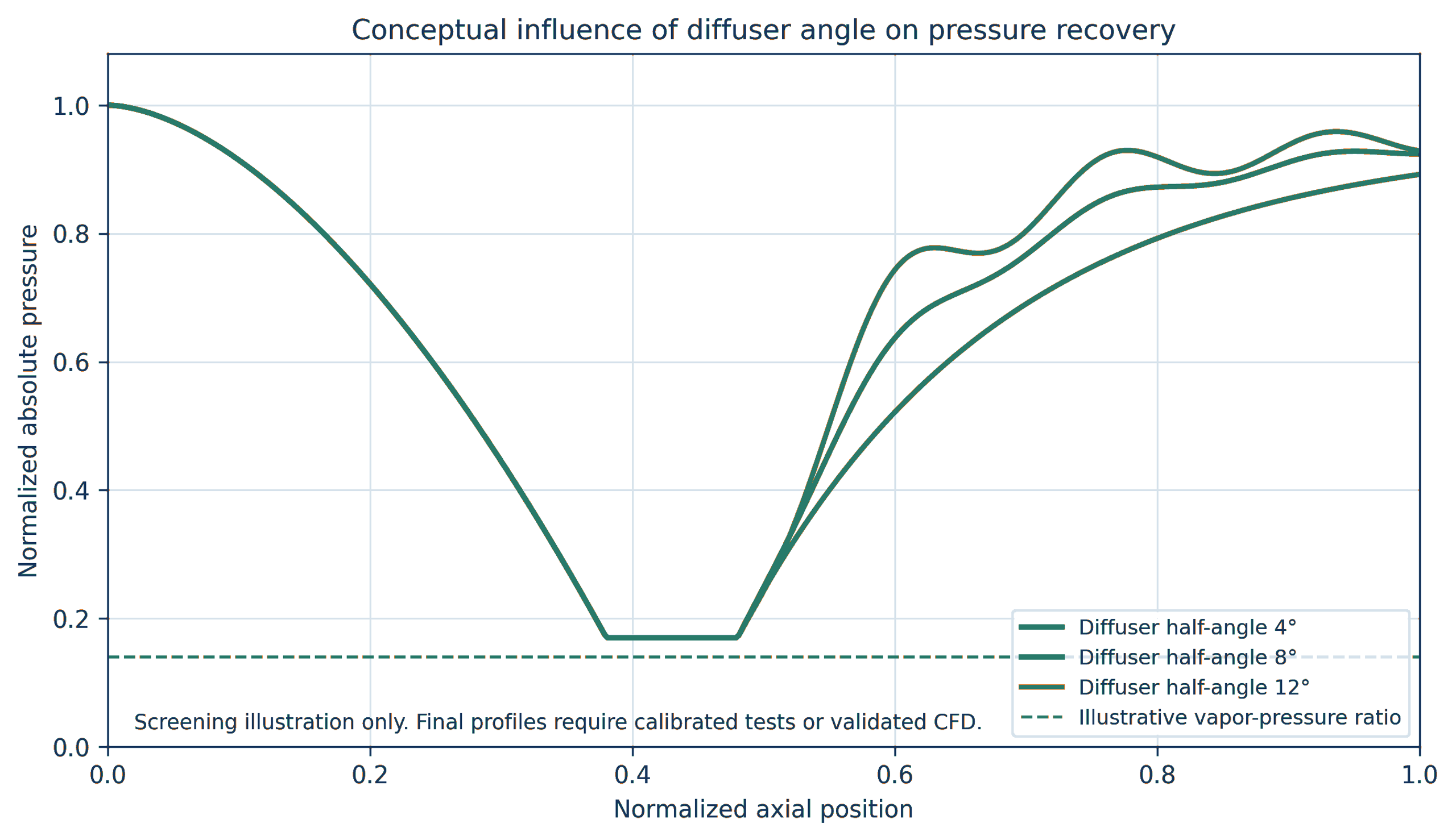
Figure 3.5. Conceptual effect of diffuser half angle on pressure recovery [32].

Worked Example 3.2: ideal throat screen

Design basis. Water at 25 °C flows at $Q=10.0$ m³/h through a 50 mm inlet. The inlet absolute pressure is 450 kPa. An ideal throat pressure target of 2.5 kPa absolute is used to screen the minimum throat area. This target is slightly below the equilibrium vapor pressure and intentionally signals that a single phase Bernoulli model has reached its limit.

The inlet velocity is 1.415 m/s. Equation (3.11) gives an ideal throat velocity of 30.0 m/s. Equations (3.10) and (3.12) give $A_t=9.26\times {10}^{-5}$ m² and $d_t=10.86$ mm. Equation (3.13) gives ${\beta }_t=0.217$.

For a return to 50 mm diameter, Equation (3.16) gives the following geometric lengths:

Table 3.3. Diffuser length screen for Worked Example 3.2.

Diffuser half angle	Calculated diffuser length
4°	0.280 m
6°	0.186 m
8°	0.139 m
10°	0.111 m
12°	0.092 m

The calculation does not imply that a 10.86 mm throat will maintain an absolute pressure of 2.5 kPa. Once vapor forms, the density field, momentum exchange, wall friction, compressibility, choking, and pressure recovery change. The calculated throat should therefore be treated as an initial geometry, followed by a realistic pressure profile obtained from a calibrated coefficient or CFD, sufficient throat length for the required cavity residence time, and testing of multiple diffuser geometries. Absolute inlet pressure must also be verified at minimum pump delivery and maximum operating temperature.

Venturi design checks

A final Venturi calculation should include:

• inlet and throat Reynolds numbers over the full viscosity range;

• contraction loss and the possibility of inlet separation;

• minimum absolute pressure and vapor fraction, not only inlet to outlet loss;

• throat residence time $L_t/V_t$;

• diffuser recovery and separation;

• downstream pressure needed to collapse cavities within a replaceable chamber;

• pressure pulsation and structural fatigue;

• throat wear, surface finish, and dimensional inspection;

• gas release and two phase choking;

• cleanability and minimum passage;

• pump curve, available suction head, and prevention of unintended pump cavitation.

3.3 Bluff body, wake, impingement, and multistage devices

A bluff body creates separated shear layers and a low pressure wake. Cavitation may form along the separation region, in periodic vortices, or where jets impinge and turn. The geometry can be a cone, cylinder, disk, wedge, baffle, liquid

whistle or opposed jet element. The global pressure drop can be represented by a loss coefficient, but useful calculation also requires blockage, wake length, shedding frequency, and the location of solid surfaces relative to collapse [2,4].

The blockage ratio is:

where $A_b$ is the projected bluff body area. Periodic wake behavior is characterized by the Strouhal number:

where $f_s$ is shedding frequency and $d_b$ is a characteristic body dimension. A measured acoustic peak should not be identified automatically as the shedding frequency because pump pulsation, structural resonance, cavity cloud oscillation, and blade or valve frequencies may overlap.

Multistage devices place several restrictions or baffles in series. The total measured loss is:

where $N_s$ is number of stages and $\mathrm{\Delta }{p}_{conn}$ includes connecting passages, expansions, and manifolds. The corresponding hydraulic power is:

Equal division of total pressure drop among stages is not guaranteed. Upstream gas release, temperature rise, changing vapor fraction, fouling, and different downstream recovery conditions can make nominally identical stages operate differently. Pressure measurements between stages or a validated model are required when stage by stage control is important.

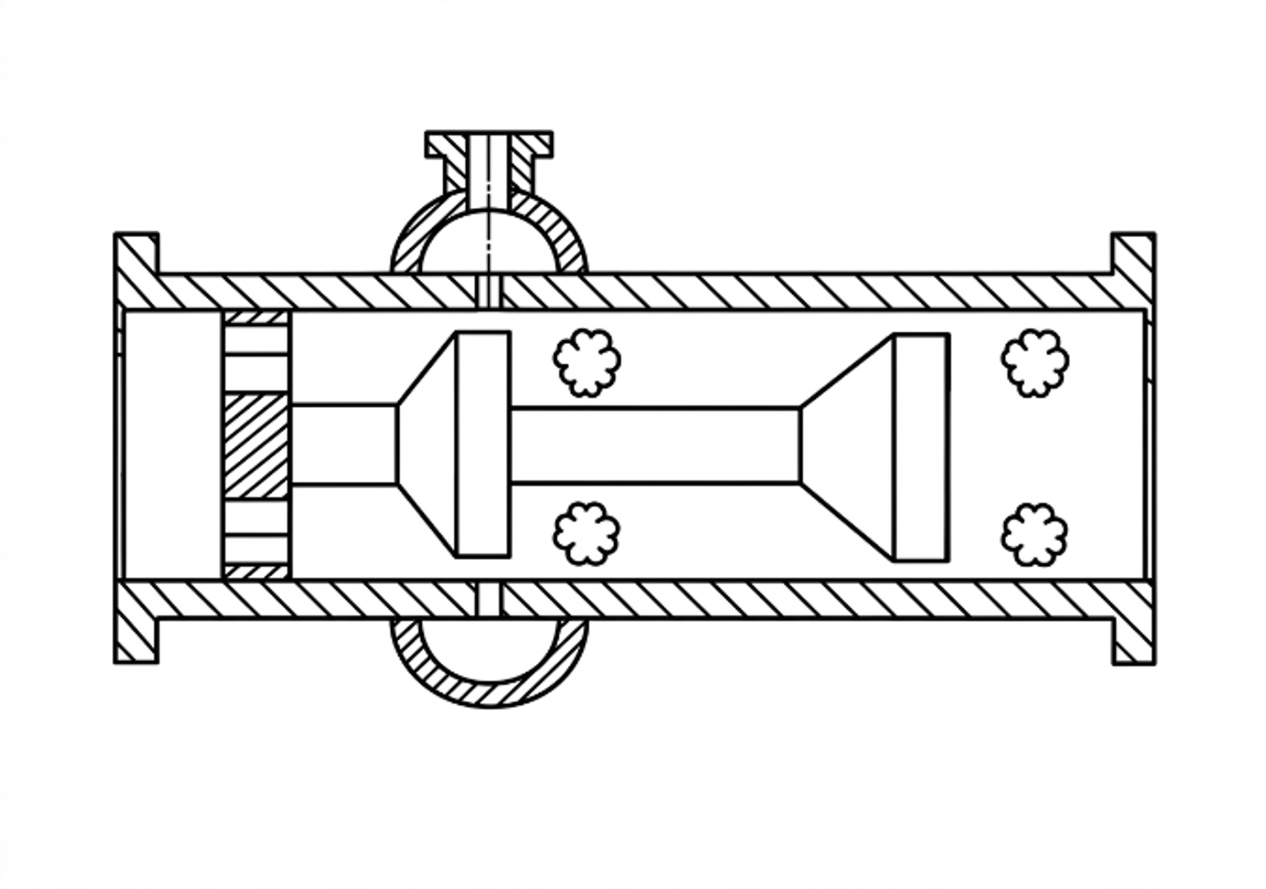
Figure 3.6. Multistage flow through cavitation device with repeated baffle elements. [13].

A multistage design should provide enough pressure recovery before the next restriction to obtain the intended collapse and regrowth sequence. If the pressure remains near vapor pressure throughout the device, the result may be a connected supercavity rather than repeated discrete collapse zones. Conversely, complete recovery at every stage can impose high cumulative pressure loss and concentrate erosion at each wall. Stage spacing, chamber diameter, baffle orientation, and intermediate pressure are therefore coupled with design variables.

Table 3.4. Calculation record for a multistage static device.

Stage	Restriction geometry	$𝐐$	${𝐩}_{𝐢𝐧}$ abs.	Estimated ${𝐩}_{\min }$ abs.	${𝐩}_{𝐨𝐮𝐭}$ abs.	$𝚫{𝐩}_{𝐢}$	Residence or spacing	Inspection feature
1	Hole, slit, cone, or baffle							Replaceable insert or coupon
2	Hole, slit, cone, or baffle							Intermediate tap
3	Hole, slit, cone, or baffle							Removable collapse chamber
$N_s$	Final element							Downstream thickness monitor

3.4 Static device scale up and scale out

Geometric enlargement of a static device changes absolute hole size, jet spacing, wall distance, residence time, pressure recovery, and the population of nuclei passing through each active zone. Keeping $\sigma$ constant does not preserve these quantities. A multi hole device can often be scaled by increasing the number of validated holes or by using parallel cartridges, but the manifold must distribute flow uniformly. A Venturi can be enlarged geometrically, but diffuser behavior and cavity length may not remain similar at a new Reynolds number and pressure scale. A bluff body device can change shedding and wake confinement as blockage and chamber dimensions change [4, 7–10].

The recommended scale up hierarchy is:

• Preserve the active geometric feature and its dimensionless ratios.

• Preserve the pressure history, including the recovery region, rather than only total pressure drop.

• Match the relevant Reynolds, Euler, Weber, and cavitation number definitions as closely as practical.

• Preserve or deliberately redesign the exposure time and number of active zones.

• Verify pressure, flow, cavity signature, product response, specific electrical energy, and material loss simultaneously.

• Prefer parallel scale out when one large device introduces a new, unvalidated flow structure.

A static device should be accepted only after the pump and piping system are considered. The cavitator may be correctly sized while the pump operates near suction cavitation, the downstream valve creates a second uncontrolled cavitation zone, or the recirculation line accumulates gas. The complete hydraulic system curve, pump curve, relief path, maximum blocked in pressure, and minimum downstream pressure belong in the calculation package.

4 Calculations for Vortex Cavitation Devices

A vortex cavitation device uses tangential momentum to establish a radial pressure gradient. The lowest mean pressure occurs near the vortex axis, allowing the principal cavity to remain within the fluid core rather than attach directly to the outer wall. This arrangement can reduce direct wall exposure, although collapse may still occur near the outlet, end plate, core stabilizer, or downstream recovery chamber. Vortex configurations include single or multiple tangential inlets, annular entries, conical or stepped chambers, vortex diodes, axial or tangential outlets, and staged or parallel modules [4, 7–10, 14].

The calculation comprises three stages. First, the tangential inlets and outlet are sized for the required flow and pressure drop. Second, a radial equilibrium model is used to screen whether circulation can reduce the core pressure toward the vapor pressure region. Third, the model is calibrated because real vortex flow contains a viscous core, axial velocity, turbulent diffusion, precession, gas release, and vapor, all of which limit the pressure depression predicted by an ideal free vortex model.

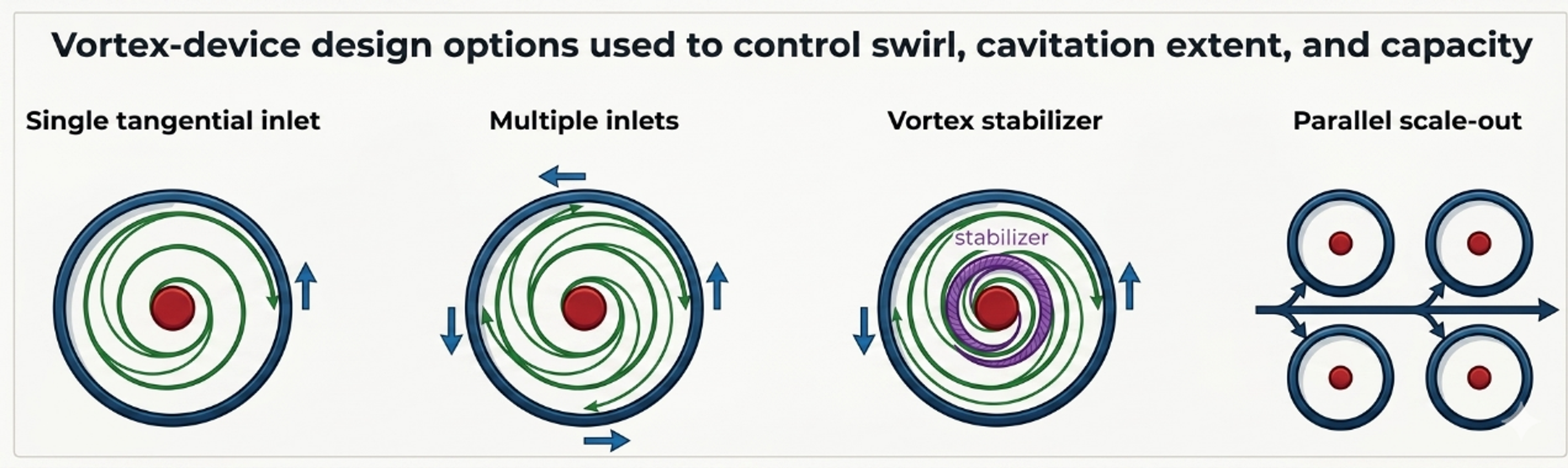
Figure 4.1. Representative vortex cavitation configurations and geometric variables [32].

4.1 Radial equilibrium screening model

For steady axisymmetric swirling flow with radial velocity small relative to tangential velocity, radial equilibrium is

where $V_{\theta }$ is tangential velocity and $r$ is radius from the axis. Outside a finite viscous core, an ideal free vortex can be represented as:

where $\mathrm{\Gamma }$ is circulation. Integrating Equation (4.1) between an outer radius $r_o$ at pressure $p_o$ and radius $r$ gives:

The mathematical free vortex predicts unbounded velocity and decreasing pressure as $r\to 0$, which is not physical. A preliminary device calculation therefore specifies a finite core radius $r_c$ and applies Equation (4.3) only for $r\ge r_c$. Inside the core, a forced vortex or measured profile is more appropriate.

The circulation required for the calculated pressure at $r_c$ to reach vapor pressure is:

Equation (4.4) is a useful screening criterion, but it does not predict the resulting vapor core radius. Once $p\le p_v$, a two phase core forms and modifies the velocity and pressure field. The criterion also depends strongly on the assumed $r_c$, which must be obtained from measurement, validated CFD, or a correlation for the selected chamber.

4.2 Tangential inlet and outlet sizing

For $N_i$ equal tangential inlets of area $A_i$, the nominal inlet velocity is:

The inlet Reynolds number should use the appropriate hydraulic diameter. Multiple inlets can improve azimuthal symmetry and distribute momentum, but their jets may interact differently as device scale, chamber aspect ratio, and inlet to chamber area ratio change.

A practical inlet velocity ratio is:

where $V_{\tan }$ and $V_{ax}$ are nominal tangential and axial velocity components at a defined station. $S_v$ is not the formal integral swirl number used in combustor analysis; it is a reproducible engineering ratio for a specific inlet geometry. When the inlet is purely tangential, the downstream axial component is generated by the outlet and internal recirculation, so it should be obtained from a mass balance or a resolved flow field.

The chamber aspect ratio is:

where $H_c$ is chamber height or axial length and $D_c$ is chamber diameter. Aspect ratio affects core residence, end wall interaction, and the distance available for vapor growth and recovery.

A vortex device Euler number based on inlet velocity is:

For a geometrically similar, calibrated vortex family, flow can be represented in the form:

where $K_v$ is an empirical capacity coefficient that contains inlet number, inlet ratio, outlet ratio, aspect ratio, and internal losses. Equation (4.9) is a family correlation, not a universal vortex law. Recent scale up studies demonstrate that device scale and geometry can change both cavitation and process response even when a global pressure drop parameter is preserved [7–10].

4.3 Outlet pressure, core stability, and recovery

The outlet must remove the required flow without suppressing the core or causing uncontrolled cavitation at an outlet edge. An undersized axial outlet increases backpressure and can shorten the vapor core; an oversized outlet may weaken the circulation or move recovery into downstream piping. An outlet tube extending into the chamber can stabilize or disturb the core depending on its diameter, insertion depth, and edge profile.

The following pressures should be distinguished:

• $p_o$, the pressure near the outer chamber radius used in a radial equilibrium model;

• $p_c$, the mean core pressure;

• $p_{out}$, the outlet pressure measured;

• $p_{\min }$, the instantaneous local minimum from a resolved model or high frequency measurement;

• $p_{rec}$, the pressure where cavity collapse is intended.

A vortex can continue to contain a gas rich or vapor rich core when the measured outlet pressure is well above vapor pressure. Conversely, low outlet pressure does not prove that the strongest collapse occurs inside the chamber. Imaging, pressure mapping, acoustic monitoring, and erosion inspection should be used together.

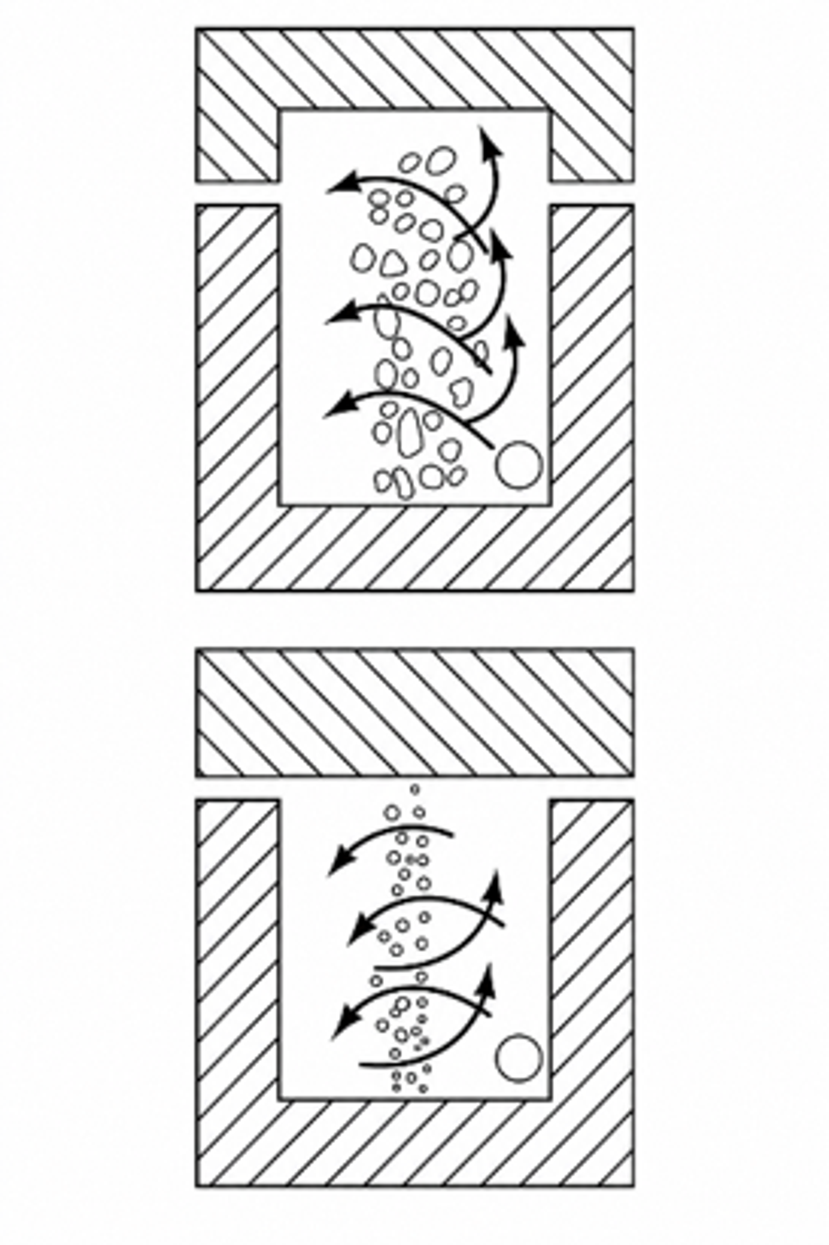
Figure 4.2. Vortex cavitation device showing tangential admission and axial core/outlet features. [14].

4.4 Worked Example 4.1: finite core vortex screen

Design basis. A water device at 25 °C has outer model radius $r_o=25$ mm, assumed finite core radius $r_c=4$ mm, and outer reference pressure $p_o=120$ kPa absolute. Four circular tangential inlets, each 4.0 mm in diameter, deliver $Q=3.0$ m³/h. Water properties are $\rho =997$ kg/m³ and $p_v=3.17$ kPa absolute. Circulation is varied to show the sensitivity of the single phase radial equilibrium model.

Equation (4.4) gives ${\mathrm{\Gamma }}_{crit}=0.390$ m²/s. Equation (4.3) gives the following core pressures:

Table 4.1. Worked Example 4.1 finite core results.

Circulation $𝚪$	Calculated $𝐩\left({𝐫}_{𝐜}\right)$ absolute	Interpretation
0.32 m²/s	41.3 kPa	Above vapor pressure in the single phase screen
0.36 m²/s	20.3 kPa	Strong pressure depression, but still above $p_v$
0.39 m²/s	3.04 kPa	Approximately the calculated inception boundary
0.42 m²/s	−15.7 kPa	Nonphysical single phase result; vapor core model is mandatory

Equation (4.5) gives a nominal velocity of 16.58 m/s in each of the four tangential inlets. The calculation does not determine the fraction of inlet momentum converted into circulation. That conversion depends on inlet orientation, wall friction, end wall flow, axial extraction, and turbulence. A measured velocity field or validated CFD is required to relate $V_i$ to $\mathrm{\Gamma }$.

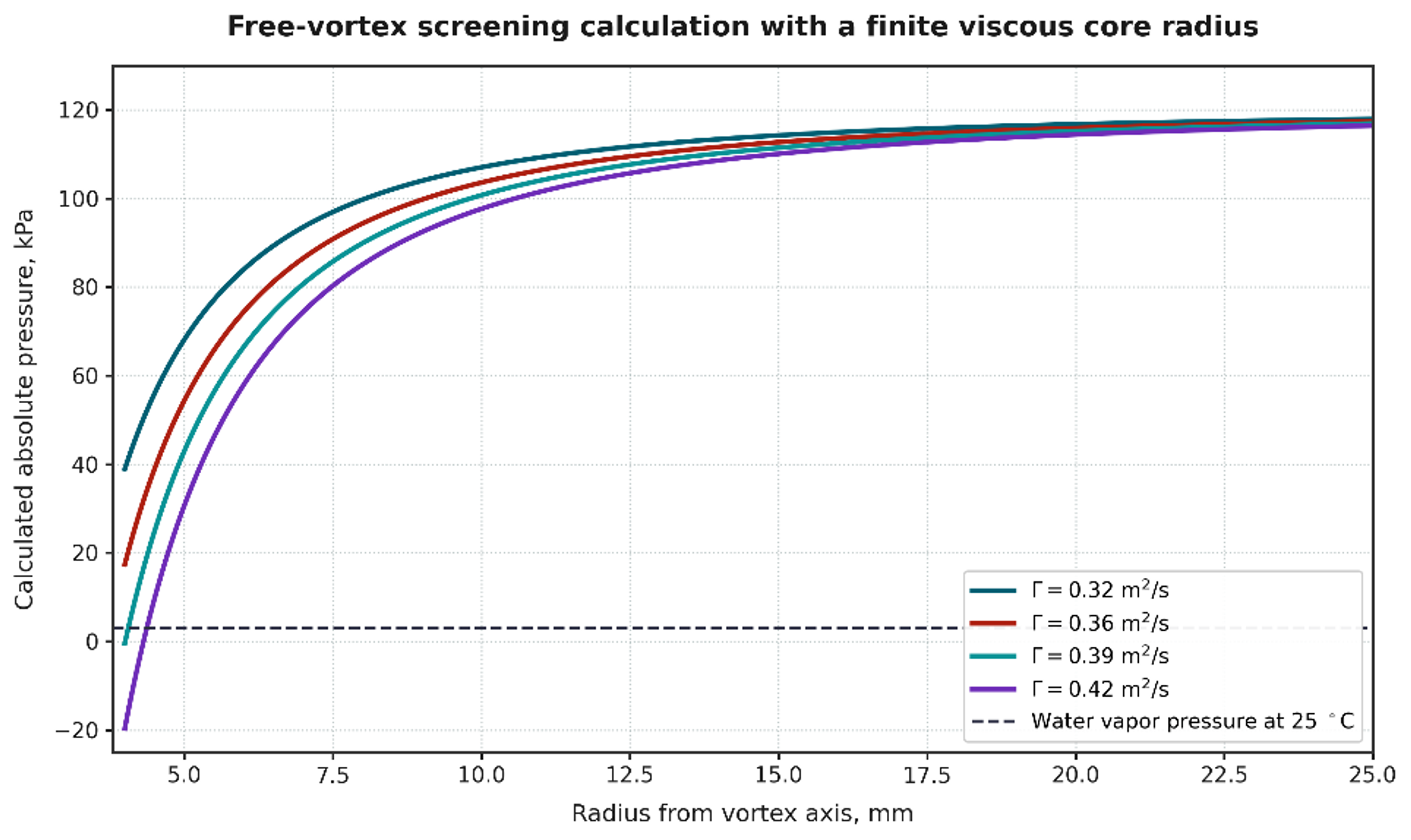
Figure 4.3. Calculated radial pressure profiles for Worked Example 4.1. Calculation using Equations (4.1) to (4.3). Where the single phase model predicts pressure below vapor pressure, a two phase cavitation model is required [32].

The worked example demonstrates two important design limits. First, the inferred core pressure is extremely sensitive to circulation and assumed core radius. Second, a negative absolute pressure from Equation (4.3) is not a prediction of a real negative pressure operating state. It indicates that the single phase model has crossed its validity boundary and must be replaced by a vapor core or multiphase model.

4.5 CFD and experimental calibration for vortex devices

A useful vortex CFD model should reproduce non cavitating pressure loss before cavitation parameters are adjusted. The mesh must resolve tangential inlets, near wall layers, outlet edges, and the core region. Transient simulation is often required because the core can precess and vapor clouds can shed. The selected cavitation model, nuclei density, bubble radius, mass transfer coefficients, turbulence model, and compressibility assumptions should be reported. Grid and time step independence should be demonstrated for pressure drop, core size, vapor volume, and dominant frequency, not only for a global residual [3, 4, 7].

Experimental calibration should include:

• a water flow pressure map at several backpressures;

• absolute pressure and temperature at every relevant station;

• visualization or a transparent development chamber where practicable;

• high frequency pressure or acoustic data to identify core precession and cloud shedding;

• flow distribution among parallel modules;

• product response versus pressure drop, passes, and scale;

• erosion or witness coupons at end walls, outlet edges, and recovery surfaces;

• repeat tests after dimensional wear to identify drift.

Studies of vortex devices for degradation and continuous emulsification show that pressure drop, number of passes, chamber geometry, device scale, dispersed phase fraction, and scale out arrangement affect performance. These results support the use of calibrated device families and parallel scale out rather than the assumption that one global cavitation number guarantees similarity [7–10].

4.6 Vortex scale up and scale out

For geometric scale up, inlet area, outlet area, chamber diameter, chamber height, and core stabilizer dimensions can be scaled by a common factor, but the absolute boundary layer thickness, viscous core, residence time, turbulence spectrum, and gas transport do not necessarily remain similar. Matching $E{u}_v$ and Reynolds number may require incompatible changes in flow and pressure. In addition, a larger chamber gives cavities more time to grow and can shift collapse toward an end wall or outlet.

Parallel scale out preserves the validated internal geometry. The manifold calculation should limit branch to branch flow variation, provide an isolation valve and pressure measurement for each module, and avoid a header pressure gradient that changes backpressure systematically across the array. The total capacity is:

where $N_m$ is number of modules. Uniformity can be reported as the coefficient of variation:

where $s_Q$ and $\bar{Q}$ are the standard deviation and mean of branch flows. The acceptable $C{V}_Q$ should be linked to the sensitivity of product performance to flow and pressure drop. A manifold that is hydraulically acceptable for ordinary heat exchange may still be too nonuniform for a narrow cavitation operating window.

Table 4.2. Vortex device calculation and validation checklist.

Item	Preliminary calculation	Calibration or acceptance evidence
Tangential inlets	Number, area, hydraulic diameter, velocity, $Re$, pressure loss	Measured branch or inlet flow and dimensional inspection
Chamber	$D_c$, $H_c$, $AR$, hold up, nominal residence time	Pressure map, visualization, residence time or tracer test
Core	$r_c$, ${\mathrm{\Gamma }}_{crit}$, calculated pressure profile	PIV, high speed imaging, CFD, acoustic or dynamic pressure signature
Outlet	Area ratio, velocity, insertion depth, recovered pressure	Stable flow pressure map and verified collapse location
Energy	$Q\mathrm{\Delta }p$, electrical input, heat balance	Calibrated electrical meter and temperature history
Scale up	$Re$, $E{u}_v$, geometry ratios, residence time	Pilot comparison at same product composition
Scale out	Header and branch losses, $C{V}_Q$, isolation	Individual branch flow or pressure confirmation
Integrity	End wall and outlet erosion screen	Coupons, thickness map, contamination analysis

5 Calculations for Dynamic Hydrodynamic Cavitation Devices

Dynamic hydrodynamic cavitation devices use rotation to generate repeated pressure depressions, wakes, gap flow, and cavity collapse. Principal configurations include rotor stator teeth, pins, perforated disks, dimpled or cavity rotors, serrated disks, high speed impellers, and rotating cylinders. Some machines combine pumping and cavitation, whereas others require an external pump to establish axial flow through the rotor chamber. Rotational speed provides an independent control variable, but the design calculation must also include shaft power, torque, clearance, rotor stress, balance, seals, bearings, vibration, and heat generation [7, 17].

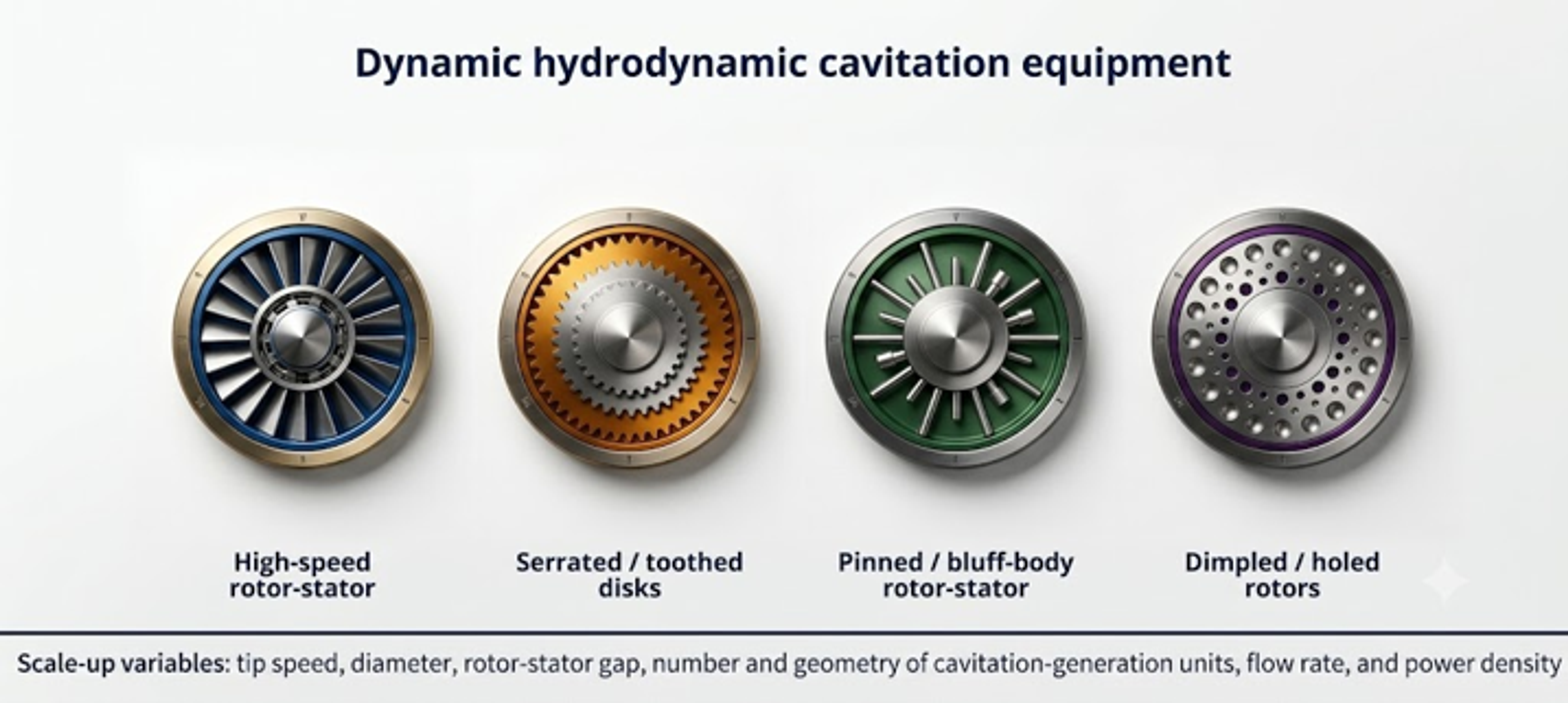
Figure 5.1. Principal dynamic hydrodynamic cavitation device families [32].

A dynamic device should not be sized by rotational speed alone. Machines operating at the same revolutions per minute can exhibit substantially different tip speeds, pressure fields, power demand, and cavitation behavior because rotor diameter, cavity geometry, clearance, flow rate, chamber pressure, and liquid properties differ. The minimum reproducible data set should include rotor and stator drawings, diameter, axial and radial clearances, number and geometry of repeating features, rotational speed, shaft power or torque, chamber pressure, flow rate, temperature, gas condition, and pressure tap locations.

5.1 Speed, tip velocity, and rotational Reynolds number

Rotational speed in revolutions per second is:

and angular velocity is:

For rotor diameter $D_r$, tip speed is:

A rotational Reynolds number convenient for similar rotors is:

A tip speed Reynolds number $\rho u_{tip}{D}_r/\mu$ can also be used, but the definition must not be changed between data sets. Because the two definitions differ by a factor of $\pi$, an unlabelled rotational Reynolds number can cause a substantial comparison error.

A rotor based cavitation number is:

where $p_b$ is a defined bulk or chamber absolute pressure. Equation (5.5) is an operating index. The local pressure in a cavity, trailing wake, stator opening, or rotor stator gap depends on the feature geometry and unsteady interaction. A geometry specific inception coefficient must be obtained experimentally or through validated CFD.

The tip Mach number is:

where $c$ is liquid sound speed. The bulk tip Mach number may be small while local pressure waves and vapor cloud collapse remain compressible phenomena. The quantity is useful for screening whether incompressible mechanical flow assumptions are reasonable outside the collapse zone.

5.2 Power number, torque, and motor sizing

The power number is:

where $P_s$ is shaft power transferred to the fluid and mechanical losses included within the selected boundary. Rearrangement gives:

The $n^3{D}^5$ dependence makes power extremely sensitive to speed and scale. Equation (5.8) is valid only when $Po$ has been calibrated for the same geometry, clearance, flow coefficient, Reynolds number region, chamber pressure, gas fraction, and rheology. Extrapolation through cavitation inception can be inaccurate because vapor changes torque and flow structure.

Shaft torque is:

The motor should be selected from the maximum required torque and power over start up, normal operation, maximum viscosity, maximum solids, cleaning, and upset conditions. A variable frequency drive must satisfy both continuous current and low speed cooling requirements. The shaft, key, coupling, and gearbox should be checked against transient torque and fatigue, not only average power.

Measured electrical power can be converted to estimated shaft power using a calibrated motor and drive efficiency, but direct torque measurement is preferable during development. Bearing, seal, windage, and drive losses under no load should be measured because they can be a substantial fraction of the total in a small laboratory unit.

5.3 Clearance, shear rate, and passage frequency

For a narrow rotor stator gap $g_c$, the first order Couette shear rate screen is:

where $u_{rel}$ is relative surface velocity. The actual field includes pressure driven flow, turbulence, leakage, entrance and exit jets, and vapor. Equation (5.10) is useful for mechanical and rheological screening but should not be interpreted as the volume averaged treatment shear rate.

If $z_f$ identical rotor features pass a stationary reference point per revolution, the blade or feature passage frequency is:

This frequency can appear in dynamic pressure, vibration, and acoustic spectra. Sidebands or subharmonics can indicate precession, rotating cavitation, cloud shedding, or mechanical modulation. The operating speed should avoid coincidence among passage frequency, shaft frequency, structural natural frequencies, and piping acoustic modes.

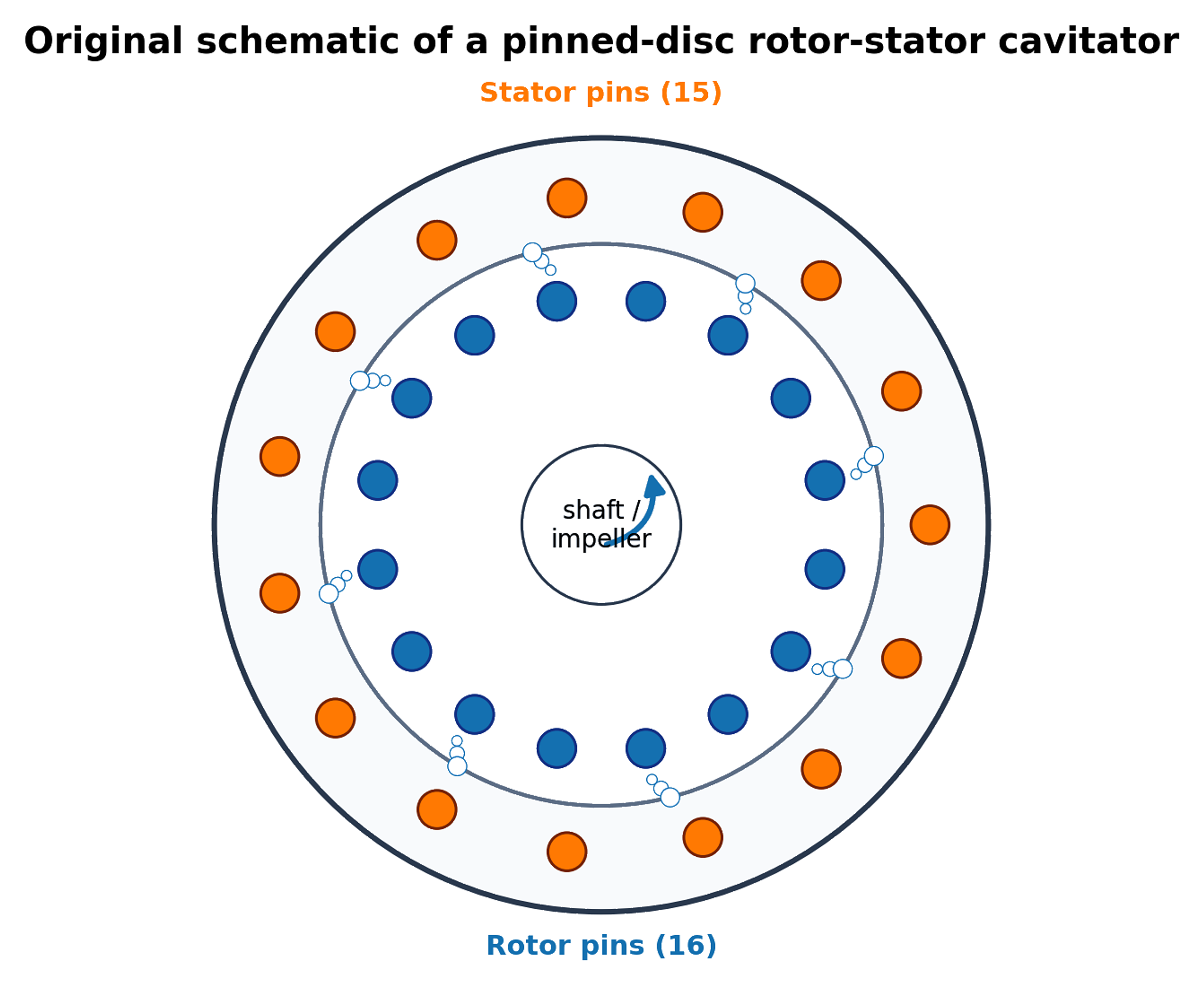
Figure 5.2. Pinned disc rotor and stator geometry and characteristic dimensions used for the worked calculation. [14, 18, 31].

5.4 Flow coefficient, pressure coefficient, and energy density

A dimensionless flow coefficient is:

and a pressure or head coefficient is:

where $\mathrm{\Delta }p$ is defined across the rotating device. Matching $Po$, $\varphi$, $\psi$, $R{e}_r$, ${\sigma }_r$, clearance ratio $g_c/D_r$, and feature ratios gives a more complete similarity basis than matching tip speed alone. In practice, exact simultaneous matching may be impossible, so pilot testing should target the most process sensitive variables.

The mass specific shaft energy for a continuous single pass is:

and an active zone power density can be defined as:

where both the power boundary and active volume must be stated. Dividing total motor input by the entire loop volume and dividing estimated local dissipation by a small gap volume produce different quantities. Both can be useful, but they must not be compared as if they were identical.

5.5 Worked Example 5.1: rotor stator operating point

Design basis. A rotor of diameter $D_r=0.190$ m operates in water at 25 °C. The selected speed is 2850 rpm, chamber pressure is 150 kPa absolute, flow is 0.0054 m³/s, gap is 0.8 mm, and the rotor has 12 repeating features. The power number $Po=0.208$ has been calibrated from a measured shaft power near 5.5 kW for this geometry and flow regime. Water properties are $\rho =997$ kg/m³, $\mu =0.00089$ Pa·s, and $p_v=3.17$ kPa absolute.

Equations (5.1) to (5.3) give $n=47.5$ s⁻¹, $\omega =298.45$ rad/s, and $u_{tip}=28.35$ m/s. Equation (5.4) gives $R{e}_r=1.92\times {10}^6$. Equation (5.5) gives ${\sigma }_r=0.366$. The low value indicates a strong rotational pressure scale, but it does not predict the local vapor fraction.

Equation (5.8) gives $P_s=5.50$ kW. Equation (5.9) gives torque $T_s=18.4$ N·m. The gap shear rate screen from Equation (5.10) is $3.54\times {10}^4$ s⁻¹, and Equation (5.11) gives a feature passage frequency of 570 Hz. Equation (5.14) gives a single pass shaft energy of approximately 1022 J/kg. The flow coefficient is $\varphi =0.0166$.

Table 5.1. Worked Example 5.1 results.

Quantity	Result	Interpretation
Rotational speed	2850 rpm; 47.5 s⁻¹	Speed must be paired with rotor diameter
Tip speed	28.35 m/s	Governs the selected rotational pressure scale
Rotational Reynolds number	$1.92\times {10}^6$	Based on $\rho n{D}_r^2/\mu$
Rotor cavitation number	0.366	Uses chamber pressure and tip speed; geometry specific calibration still required
Calibrated power number	0.208	Applicable only to the tested geometry and regime
Shaft power	5.50 kW	Excludes motor and drive losses unless calibrated otherwise
Shaft torque	18.4 N·m	Basis for coupling and shaft checks, with service factor
Gap shear rate screen	$3.54\times {10}^4$ s⁻¹	Couette estimate, not a resolved local field
Passage frequency	570 Hz	Compare with vibration and acoustic spectra
Flow coefficient	0.0166	Required for similarity comparisons
Single pass shaft energy	1.02 kJ/kg	Relates energy to continuous throughput

Using the same calibrated $Po$ without changing geometry or flow regime gives approximately 1.25 kW at 1740 rpm and 2.86 kW at 2290 rpm. The cubic speed dependence is shown in Figure 5.3. These predictions should be checked against measured torque because $Po$ can change with flow coefficient, clearance, vapor fraction, and rheology.

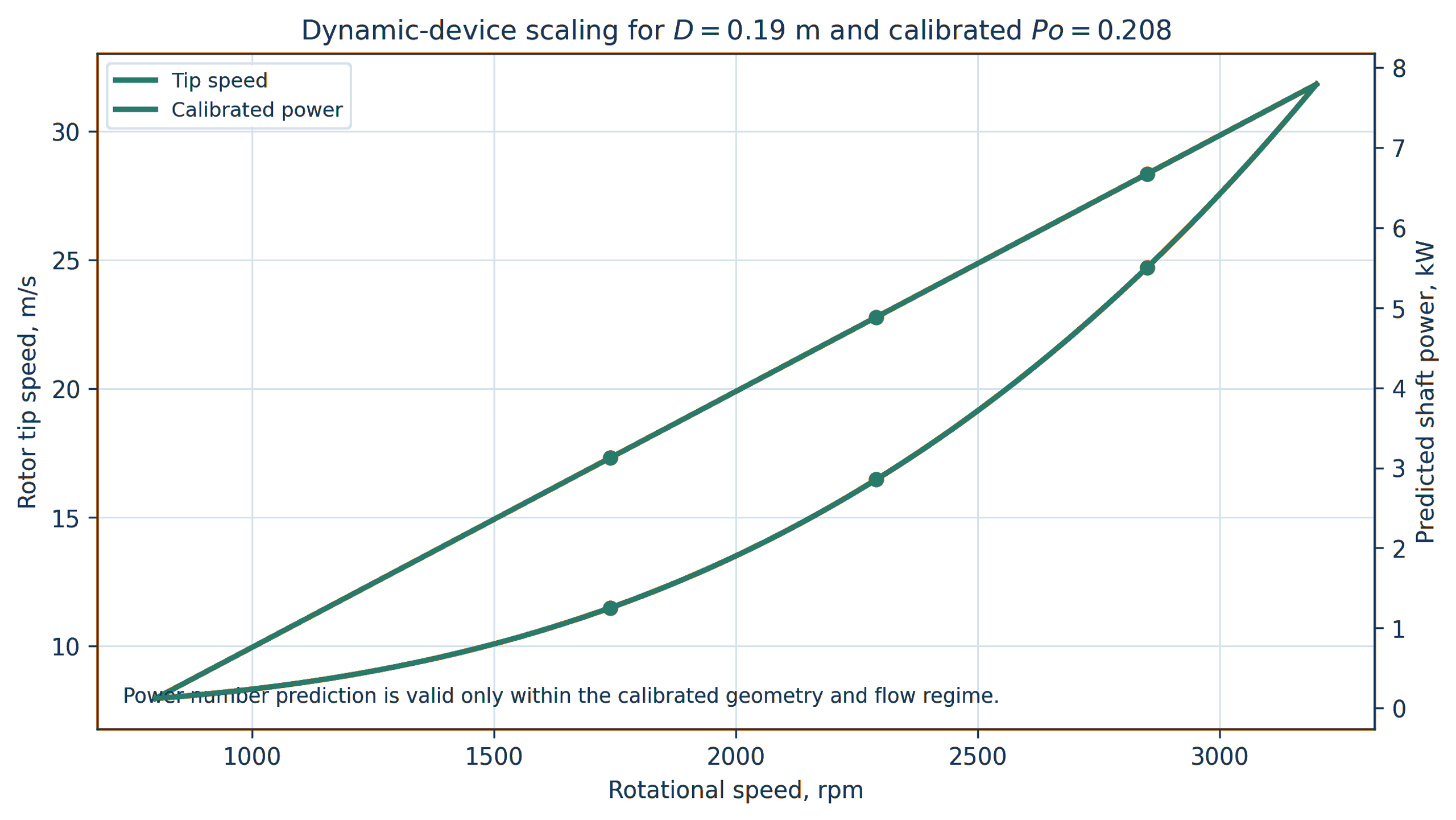
Figure 5.3. Tip speed and shaft power versus speed for Worked Example 5.1 using D_r = 0.19 m and calibrated Po = 0.208. Calculation. Power number extrapolation is valid only within the calibrated geometry and flow regime [32].

5.6 Clearance budget and mechanical tolerance

A small clearance can increase velocity gradients and rotor stator interaction, but it creates a mechanical tolerance problem. The minimum running gap must exceed the combined effects of rotor and stator manufacturing tolerance, shaft runout, bearing clearance, assembly eccentricity, rotor deflection, pressure deformation, thermal expansion, transient vibration, and allowable wear. A practical clearance budget can be written:

where every term is a one sided radial or axial allowance defined for the actual stack up. Statistical tolerance methods may be used for independent manufacturing variables, but worst case combinations are appropriate where rotor contact has severe consequences.

Thermal growth must be calculated for the rotor, shaft, housing, and stator using their temperatures and coefficients of thermal expansion. The rotor can heat faster than the housing during start up, while a cold clean in place rinse can reverse the gradient. The gap should be verified at assembly temperature, normal operation, maximum process temperature, and cleaning transitions.

5.7 Rotor stress, balance, and critical speed

For a thin free ring, a first order circumferential stress screen is:

where ${\rho }_s$ is rotor material density. Real disks, pins, holes, cavities, keys, hubs, and welds require a detailed rotating stress solution. Stress concentration, low and high cycle fatigue, corrosion fatigue, residual stress, overspeed, and loss of material by erosion must be included. Finite element analysis should use the minimum remaining section after the specified inspection interval.

Rotors should be dynamically balanced in the final assembly condition, including pins, fasteners, coatings, and replaceable elements. Cavitation erosion can change balance during service. Vibration monitoring should include shaft frequency, feature passage frequency, bearing frequencies, and broadband cavitation content. A speed sweep should identify structural resonances before prolonged cavitating operation.

5.8 Cleanability, disassembly, and wear components

A device designed for viscous, fibrous, food, pharmaceutical, or fouling service requires access to the active geometry. Replaceable rotors, stator rings, wear plates, and collapse inserts can reduce lifecycle cost and prevent the pressure boundary from becoming a sacrificial surface. Disassembly should preserve alignment and repeatable clearance. Crevices, blind holes, gasket intrusion, and trapped pressure must be eliminated or controlled.

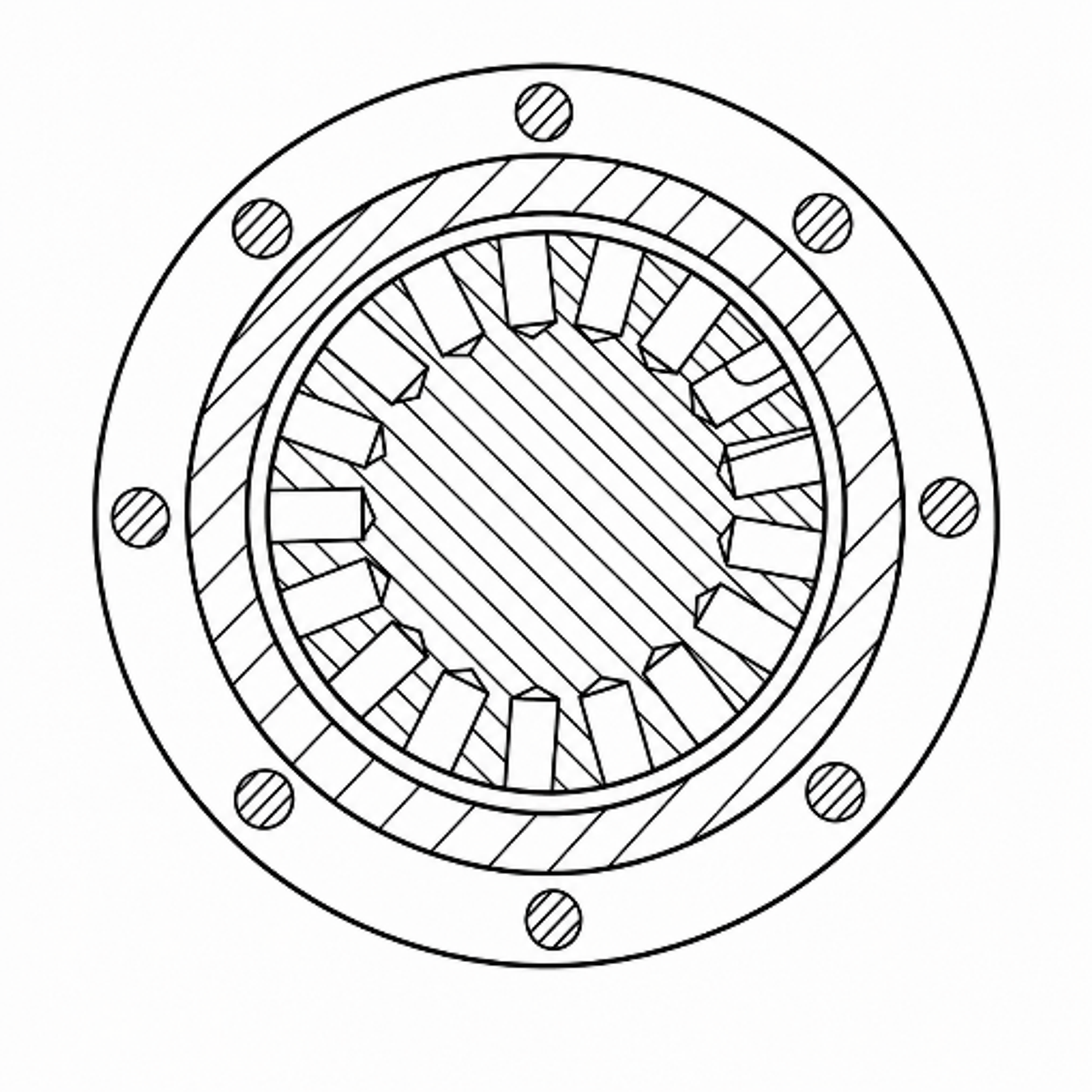
Figure 5.4. Holed rotor controlled cavitation device arranged for disassembly and cleaning. [18].

5.9 Dynamic device calculation workflow

The recommended workflow is:

• Define flow, pressure, temperature, rheology, gas, solids, product objective, and hygienic requirements.

• Select rotor diameter, feature family, number of features, chamber volume, and preliminary clearance.

• Calculate tip speed, $R{e}_r$, ${\sigma }_r$, $\varphi$, feature passage frequency, and mechanical clearance budget.

• Obtain a non cavitating torque and flow map over speed and flow.

• Identify cavitation inception using pressure, acoustic, vibration, visualization, and power changes.

• Fit $Po$ and any geometry specific inception or pressure coefficient within the validated region.

• Measure product response and temperature at the same operating points.

• Complete rotor stress, shaft, bearing, seal, pressure boundary, fatigue, overspeed, and balance calculations.

• Run an endurance test with dimensional inspection, vibration trending, and contaminant analysis.

• Scale by a defined similarity set or preserve the validated rotor module through parallel scale out.

Table 5.2. Required dynamic device calculation outputs.

Discipline	Required output
Hydraulics	Flow pressure map, chamber absolute pressure, inlet and outlet losses, residence time
Rotation	Speed range, tip speed, $R{e}_r$, $\varphi$, $\psi$, ${\sigma }_r$, passage frequency
Power	No load loss, shaft torque, $Po$, electrical input, specific energy, heat balance
Mechanical	Rotor and shaft stress, overspeed margin, critical speeds, balance grade, clearance stack up
Tribology	Seal face condition, bearing load, lubricant isolation, galling and rub assessment
Process	Product response surface, temperature history, gas condition, pass or staging dependence
Integrity	Erosion map, minimum remaining thickness, vibration trend, metal contamination
Sanitary design	Surface finish, drainability, clean in place coverage, disassembly validation

6 Selection of Structural Materials

Structural material selection for a cavitation device cannot be reduced to a single alloy ranking. The pressure boundary, cavitation generating insert, rotor, shaft, wear plate, fastener, seal face, gasket, and product contact surface perform different functions. Pressure retaining walls require weldability and code allowable stress; removable inserts require erosion resistance and dimensional stability; rotors require fatigue strength and balance; and sanitary surfaces require corrosion resistance, cleanability, low metal release, and controlled finish. Assigning all functions to one material can increase cost while reducing lifecycle performance [22–27].

The preferred design strategy first controls the hydraulic collapse location, then assigns replaceable wear components, and only afterward considers alloy or coating upgrades. No practical material is immune to sufficiently aggressive cavitation. A hard surface may resist plastic indentation but fail by brittle cracking or coating delamination. A corrosion resistant alloy can repeatedly lose its passive film under impact, while a tough alloy may deform and work harden but release metal. Material selection must therefore reflect the actual chemistry, temperature, solids, gas content, pressure history, geometry, permitted contamination, and inspection interval [23–25].

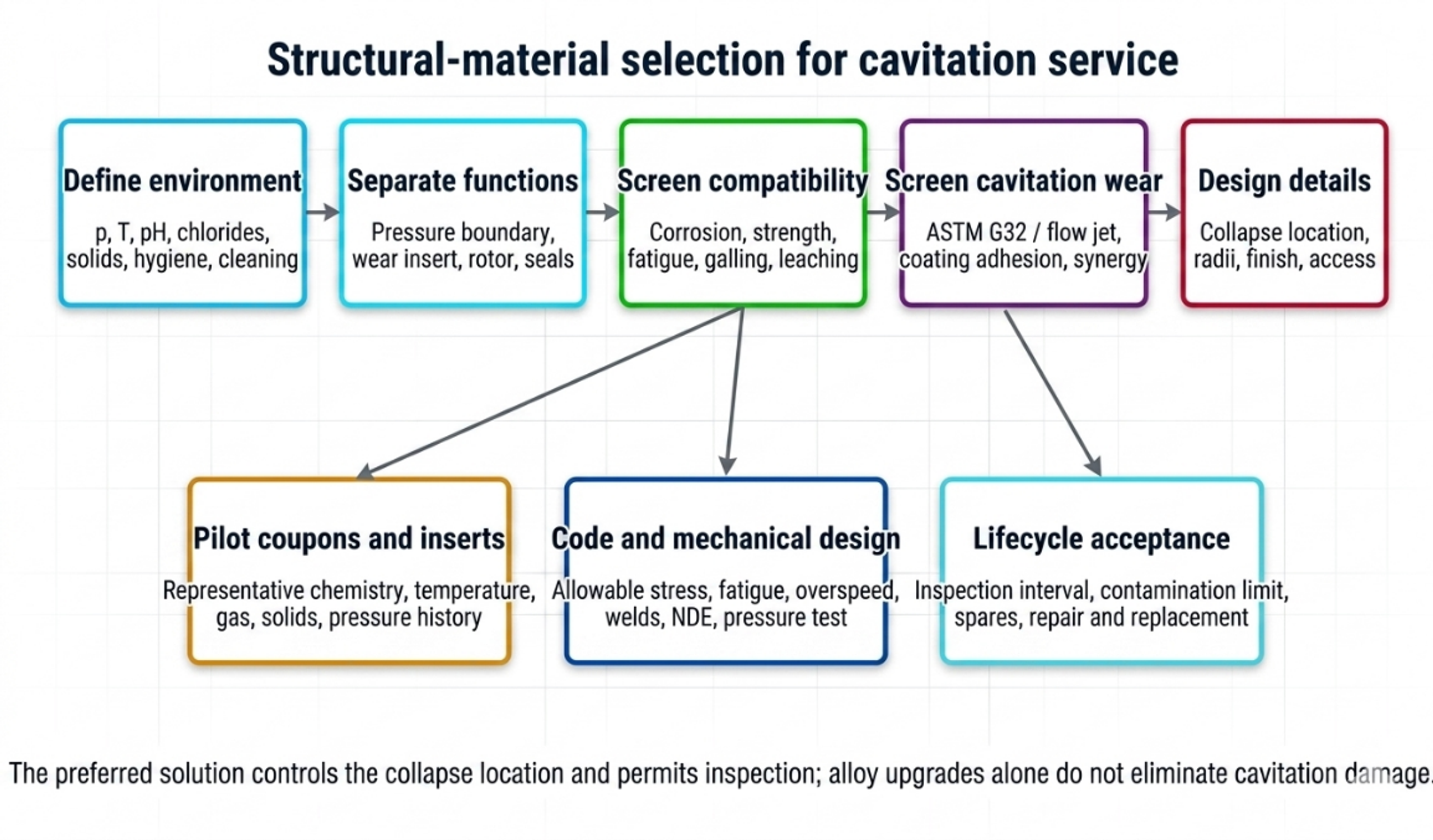
Figure 6.1. Structural material selection workflow for hydrodynamic cavitation equipment [32].

6.1 Functional decomposition of the device

The calculation package should identify the material function of every component:

Pressure boundary: contains maximum allowable working pressure, relief pressure, vacuum, thermal load, and piping reaction.

Cavitation insert or throat: defines the hydraulic geometry and may be intentionally replaceable.

Collapse chamber or wear plate: receives the highest expected microjet and cloud collapse loading.

Rotor and shaft: resist centrifugal stress, torque, fatigue, corrosion, and erosion while maintaining balance.

Stator and clearance surfaces: maintain geometry under pressure, temperature, and possible rub.

Seals, gaskets, and bearings: remain compatible with chemistry and temperature while preventing product contamination.

Welds and heat affected zones: meet pressure code, corrosion, fatigue, and surface finish requirements.

Instrumentation connections: avoid crevices, dead legs, thin diaphragms exposed to collapse, and plugged impulse lines.

A replaceable insert allows the pressure shell to be selected primarily for code, corrosion, and fabrication, while the wear component is selected for cavitation exposure. The insert should have positive location, repeatable dimensions, no bypass leakage, and an inspection datum. Its failure must not release a loose part into downstream equipment.

6.2 Pressure boundary screening

For a cylindrical wall under internal pressure, a simplified thin wall screen can be written:

where $p$ is design pressure, $D$ is the selected diameter basis, $S$ is allowable stress, and $E$ is weld joint efficiency. Equation (6.1) is only a preliminary screen. Final thickness, reinforcement, flange rating, fatigue, external pressure, nozzle loads, weld details, examination, testing, and material allowable must comply with the applicable pressure vessel or piping code, such as ASME BPVC Section VIII or ASME B31.3 [26, 27].

A practical nominal thickness expression is:

where $t_{code}$ is code required thickness, $c_{corr}$ is corrosion allowance, $c_{eros}$ is a justified erosion allowance, $c_{mach}$ is machining or resurfacing allowance, and $m_t$ is the negative mill tolerance fraction. An erosion allowance should not replace inspection or a wear insert when cavitation attack is localized.

Worked structural screen

For $p=1.6$ MPa, $D=0.100$ m, $S=115$ MPa, and $E=0.85$, Equation (6.1) gives $t_s=0.825$ mm. This small value illustrates only membrane pressure demand. It is not a final wall thickness. A real device may require substantially more thickness for code minimums, threading, nozzles, flange loads, cyclic pressure, vibration, manufacturing tolerance, corrosion, erosion, and rigidity needed to preserve a small internal clearance.

6.3 Cavitation erosion and erosion corrosion interaction

Cavitation erosion is produced by repeated pressure pulses, microjets, cloud collapse, and associated cyclic deformation. The incubation period may show little measurable mass loss while subsurface fatigue accumulates. It can be followed by an accelerating stage, a maximum rate, and a later rate modified by roughness and the evolving flow. A single test duration can therefore misrepresent long term behavior [23, 24].

ASTM G32 provides a vibratory apparatus method for comparative cavitation erosion testing [23]. Its output is valuable for screening materials, heat treatments, and coatings under controlled conditions, but it should not be converted directly into plant service life. A hydrodynamic device has different impact frequency, bubble cloud scale, pressure recovery, chemistry, temperature, solids, and wall geometry. The strongest program combines standardized comparison, a representative flow test, and pilot inserts in the actual process.

Mean depth of erosion calculated from mass loss is:

where $\mathrm{\Delta }m$ is mass loss, ${\rho }_s$ is solid density, and $A_e$ is exposed area. The mean depth penetration rate is:

A combined erosion corrosion loss may be expressed conceptually as:

where $W_{cav}$ is purely mechanical cavitation loss, $W_{corr}$ is corrosion loss without cavitation, and $W_{syn}$ is the interaction term. The interaction can be positive because impact removes passive films and corrosion weakens the surface, but the sign and magnitude must be measured for the actual environment [24].

For an observed approximately linear penetration rate after incubation, a remaining life screen is:

where $h_{allow}$ is the maximum permitted local penetration and $h_{meas}$ is measured penetration. This calculation is valid only when the rate is stable and the measured location corresponds to the most severe attack. Local pits or crack like defects may govern before average depth.

6.4 Material property requirements

Cavitation resistance is influenced by hardness, yield strength, strain hardening, toughness, fatigue behavior, elastic modulus, microstructure, residual stress, phase stability, corrosion resistance, surface finish, and defect population. No single property predicts performance across all regimes. The desired combination is a surface that resists repeated indentation and cracking, a substrate that supports the surface without excessive deformation, and a chemistry that maintains passivity or avoids rapid dissolution [24, 25].

Material screening should consider:

Strength and fatigue: pressure cycles, rotor stress, passage frequency loading, and vibration.

Toughness: resistance to crack initiation and propagation under repeated impact.

Hardness and work hardening: resistance to plastic indentation, with attention to brittle failure.

Corrosion: uniform corrosion, pitting, crevice corrosion, stress corrosion cracking, galvanic coupling, and corrosion fatigue.

Fabrication: weldability, heat treatment, distortion, machinability, repair, and nondestructive examination.

Surface condition: roughness, inclusions, machining marks, weld profile, coating defects, and residual stress.

Process compatibility: extractables, toxic metal limits, food or pharmaceutical conformity, product discoloration, and catalyst poisoning.

Lifecycle: cost, lead time, replaceability, inspection method, and disposal or repair.

6.5 Candidate metallic materials

Table 6.1. Qualitative material selection matrix for cavitation devices.

Material family	Potential role	Principal advantages	Principal cautions
Carbon and low alloy steel	External pressure shell or nonhygienic benign service	Low cost, strength, weldability, code familiarity	Corrosion products, product contamination, localized erosion corrosion, coating dependence
304L austenitic stainless steel	Mild sanitary or water service	Fabricability, cleanability, availability	Lower chloride pitting margin than Mo bearing grades; not immune to cavitation
316L austenitic stainless steel	Common hygienic pressure boundary and wetted components	Weldability, cleanability, improved pitting resistance over 304L	Can pit or crevice corrode in hot chlorides; moderate hardness; erosion can remove passive film
Duplex stainless steel 2205	Higher strength chloride service, pressure parts, selected rotors	Higher strength and chloride resistance than common austenitic grades	Phase balance and welding control; surface finishing and hygienic qualification require care
Super duplex or high alloy austenitic steel	Severe chloride or oxidizing aqueous service	High pitting and crevice corrosion resistance	Cost, fabrication control, availability, possible over specification if erosion dominates
Martensitic or precipitation hardening stainless steel	Shafts, rotors, replaceable wear parts	Higher strength and hardness after heat treatment	Lower corrosion resistance in some chemistries; heat treatment control; not automatically suitable for sanitary contact
Nickel base corrosion resistant alloy	Strong acids, mixed chemicals, severe corrosion	Broad corrosion resistance in selected environments	High cost, galling, density, weld procedure, chemistry specific limitations
Titanium alloy	Chloride rich service, low density rotor or wetted component	Low density and strong passive behavior in many chloride environments	Galling, galvanic coupling, hydrogen effects, fabrication cost; cavitation resistance remains condition dependent
Cobalt base or nickel base hard facing	Local replaceable wear surface	Hardness, work hardening or high temperature wear capability	Cracking, dilution, repair, cost, possible metal release restrictions
Copper alloy	Specialized marine or antimicrobial service	Thermal conductivity and selected seawater applications	Metal release, galvanic effects, chemistry limitations, generally unsuitable where copper contamination is unacceptable

The table is a screening matrix, not a substitution rule. The specific grade, product form, heat treatment, weld, surface finish, and service chemistry determine performance. Material certificates and positive material identification should be tied to the component drawing.

6.6 Coatings, surface treatments, and claddings

Coatings can increase surface hardness or corrosion resistance while retaining a tough structural substrate. Candidate technologies include physical vapor deposited nitrides, high velocity oxy fuel coatings, weld overlays, laser cladding, nitriding, shot peening, and engineered surface remelting. A recent study of CrN coated 316L illustrates that coating architecture can improve comparative cavitation behavior, but the result depends on adhesion, residual stress, porosity, substrate support, and the test environment [25].

A coating qualification should include:

• substrate grade, heat treatment, and surface preparation;

• coating composition, thickness, hardness, porosity, and residual stress;

• adhesion and edge condition;

• cavitation test before and after chemical exposure;

• thermal cycle and clean in place compatibility;

• inspection method for pinholes, cracks, and delamination;

• permitted particle or metal release;

• repair procedure and dimensional effect.

A very hard thin coating on a compliant substrate can crack when repeated pressure pulses deform the substrate. A thick sprayed coating can contain pores and reduce a small hydraulic clearance. Coating a sharp orifice edge can change its radius and discharge coefficient. The final hydraulic geometry should therefore be measured after coating.

6.7 Ceramics and cermets

Technical ceramics and cermets offer high hardness and corrosion resistance but are sensitive to tensile stress, impact defects, thermal shock, and attachment details. They are better suited to compressively supported inserts, sleeves, nozzles, or tiles than to complex unsupported pressure boundaries. A ceramic insert should have generous radii, controlled interference or compliant support, and protection against assembly impact. The consequences of fragment release must be considered for food, pharmaceutical, turbine, membrane, and precision downstream equipment.

Tungsten carbide and chromium carbide systems may be used as bulk inserts or sprayed coatings, but binder chemistry and galvanic behavior must match the process. Hardness alone does not guarantee cavitation life because binder removal, pore attack, and brittle grain pullout can control failure.

6.8 Elastomers, polymers, seals, and bearings

Elastomer selection is governed by the complete fluid mixture, temperature, pressure, cleaning chemicals, oxidants, solvent swelling, gas decompression, and regulatory status. EPDM, FKM, FFKM, nitrile, silicone, and PTFE based materials have distinct compatibility envelopes; no generic ranking is valid for all cavitation applications. Compatibility should be confirmed using supplier data and immersion or compression testing in the actual process and cleaning fluids.

Seals should be located away from the strongest collapse zone and pressure pulsation where possible. A dynamic seal calculation should include chamber pressure, shaft speed, heat generation, face loading, flush plan, solids, gas, and dry running risk. Double mechanical seals or barrier systems may be required when product containment, air exclusion, or hazardous chemistry governs. Bearings should be isolated from process liquid unless they are specifically designed as product lubricated components.

Thermoplastics can be useful for transparent development chambers, low pressure inserts, or corrosion isolation, but pressure rating, creep, solvent compatibility, temperature, ultraviolet exposure, and brittle fracture must be checked. A transparent chamber used for visualization should have a protective enclosure and a defined service life.

6.9 Hygienic and cleanable construction

Food and pharmaceutical devices should use cleanable geometry, compatible product contact materials, controlled surface finish, drainability, and validated cleaning. Inline rotor stator equipment may be evaluated against applicable 3-A requirements, but the owner remains responsible for the complete installation, including piping, seals, instrumentation, and cleaning cycle [22].

Important design details include:

• continuous welds with controlled penetration and ground or polished product surfaces where required;

• no gasket intrusion into the flow path;

• elimination of dead legs and unvented high points;

• drainable housings and sample ports;

• accessible or validated internal cavities;

• surface finish measurement after fabrication and repair;

• avoidance of threaded product contact joints unless specifically accepted;

• material and elastomer traceability;

• verification that wear debris cannot exceed product contamination limits.

Cavitation can increase cleaning action locally but does not prove that every surface receives chemical concentration, temperature, velocity, and time sufficient for cleaning. A clean in place study should use riboflavin, conductivity, temperature mapping, swabs, microbiology, or another validated method appropriate to the process.

6.10 Welds, residual stress, and fabrication quality

Weld toes, undercut, incomplete penetration, porosity, inclusions, abrupt section changes, and rough repairs can become preferred sites for cavitation attack or corrosion. Welding also changes microstructure and residual stress. Pressure boundary welds require qualified procedures, welder qualification, examination, and code acceptance. Wetted welds may require grinding, polishing, passivation, pickling, or electropolishing depending on alloy and service.

For duplex stainless steels, heat input and interpass temperature affect phase balance and corrosion performance. For precipitation hardening or martensitic grades, welding and postweld heat treatment can alter strength and corrosion resistance. For hardfacing and cladding, dilution and cracking must be controlled. Fabrication records should therefore be part of the material selection calculation package, not a separate purchasing detail.

6.11 Inspection, monitoring, and lifecycle acceptance

Inspection should concentrate on predicted collapse zones and high stress regions. A post fabrication baseline should include dimensional measurement, surface photography, mass of removable inserts, ultrasonic thickness where applicable, rotor balance, vibration, and surface finish. Initial follow up intervals should be conservative and may be extended only after a stable wear trend has been demonstrated.

Table 6.2. Inspection methods by component and damage mechanism.

Component or concern	Baseline measurement	In service indicator	Outage inspection
Orifice or throat	Diameter, edge radius, $C_d$ curve	Drift in flow pressure relation	Optical metrology, replica, mass or profile loss
Collapse chamber	Thickness map, surface photograph	Metal concentration, acoustic change	UT grid, 3D scan, dye penetrant where appropriate
Rotor	Dimensions, balance, runout, vibration	Vibration and power trend	NDE, mass, balance, crack and erosion inspection
Stator and pins	Clearance and feature geometry	Torque or pressure drift	Coordinate measurement, surface inspection
Coating	Thickness, adhesion, defect map	Metal or particle release	Microscopy, holiday or adhesion test as applicable
Pressure shell	Code examination and pressure test	Leak, strain, pressure cycle count	UT, surface NDE, weld examination
Seal and bearings	Leakage, temperature, vibration	Trend alarms	Face, sleeve, bearing and lubricant inspection

An acceptance criterion should specify maximum dimensional change, maximum local penetration, maximum vibration, allowable metal concentration, minimum remaining pressure thickness, rotor balance tolerance, and product quality limits. Replacement should be based on the governing criterion rather than waiting for leakage or catastrophic loss of geometry.

6.12 Material selection decision record

The material decision should be recorded in a table that connects service environment, failure mode, selected material, protective feature, inspection, and spare strategy.

Table 6.3. Example material decision record.

Component	Service and dominant risk	Selected construction	Design control	Verification
Pressure housing	Internal pressure, chloride bearing aqueous liquid	Code listed corrosion resistant alloy	Code thickness, corrosion allowance, qualified welds	Material certificates, NDE, pressure test, UT baseline
Orifice insert	High local velocity and edge erosion	Hardened or coated replaceable insert compatible with product	Positive location, minimum ligament, measured final edge	Flow calibration, dimensional inspection, spare insert
Collapse liner	Cloud collapse and metal release limit	Replaceable corrosion resistant wear sleeve	Move collapse away from pressure shell	Mass and 3D profile at defined intervals
Rotor	Centrifugal stress, fatigue, cavitation, balance	High strength corrosion resistant alloy with qualified heat treatment	Overspeed and fatigue analysis, generous radii	Material traceability, NDE, balance, vibration trend
Stator	Gap integrity and erosion	Tough corrosion resistant alloy or replaceable ring	Clearance budget and anti-galling pair	Gap measurement and contact inspection
Seal	Chemistry, speed, gas, cleaning	Supplier qualified face and elastomer combination	Flush or barrier plan, temperature monitoring	Leak test, compatibility record, planned replacement

The decision record should be revised when process chemistry, cleaning agent, operating temperature, pressure, speed, solids, or allowable contamination changes. A successful material in a water trial cannot be assumed suitable for a chloride, oxidant, acid, caustic, solvent, or abrasive slurry without additional evidence.

7 Integrated Design, Scale Up, and Commissioning Procedure

The calculation of a cavitation device should culminate in an integrated operating envelope rather than a single design point. Flow, inlet pressure, backpressure, temperature, speed, gas content, viscosity, solids loading, and number of passes interact. The acceptable operating region is the intersection of cavitation performance, product response, power, temperature, mechanical integrity, cleanability, and material loss constraints.

7.1 Calculation sequence

A complete design sequence is as follows:

Define the process objective. State the required transformation and quantitative acceptance variables, including distributions rather than only averages where relevant.

Define the feed envelope. Tabulate density, viscosity or rheology, vapor pressure, gas condition, solids, surface tension, corrosive species, and temperature at minimum, normal, and maximum conditions.

Define the system boundary. Identify whether power is hydraulic, shaft, or electrical; whether energy is reported per pass, per batch, per unit mass, or per product output; and whether the pump is included.

Select the cavitation mechanism. Choose a restriction, Venturi, wake, multistage arrangement, vortex chamber, or dynamic rotor according to flow, passage size, control range, cleanability, and maintenance.

Complete the preliminary hydraulic calculation. Determine areas, velocities, $Re$, $Eu$, $We$, pressure profile, $\sigma$, residence time, power, and expected recovery location.

Complete the mechanical screen. Calculate pressure boundary demand, rotor stress where applicable, clearance, torque, supports, thermal growth, and pressure cycle or speed cycle requirements.

Allocate materials by function. Separate pressure boundary, wear insert, collapse liner, rotor, stator, seal, and product contact requirements.

Calibrate the equipment coefficients. Measure $C_d$, recovery coefficient, $K_v$, $Po$, and other geometry specific quantities on the actual or a rigorously similar unit.

Map cavitation and process response. Vary pressure drop or speed, flow, backpressure, temperature, gas, and passes. Record both hydraulic state and product response.

Validate the uncertain model. Use CFD, visualization, dynamic pressure, acoustic data, tracer tests, or wear coupons according to the unresolved design question.

Run an endurance test. Confirm power, temperature, vibration, erosion, corrosion, fouling, cleanability, and product contamination.

Freeze the operating envelope and inspection interval. Define controls, alarms, dimensional limits, spare parts, and recalibration after wear or maintenance.

7.2 Operating map

A useful operating map contains, at minimum, flow on one axis and pressure drop or rotational speed on the other. Contours or labels identify:

• no or weak cavitation;

• inception and intermittent cavities;

• developed useful operating region;

• connected or supercavitating region where collapse may be displaced;

• excessive temperature rise;

• power or torque limit;

• vibration or noise limit;

• product quality acceptance region;

• erosion or contamination limit.

The optimum operating condition is application specific. The largest visible vapor cloud does not necessarily correspond to maximum reaction rate, breakup, disinfection, or energy efficiency. A stable connected cavity can reduce the number of discrete collapse events, whereas excessive backpressure can suppress useful cavity growth. The operating map should therefore be defined by the measured process objective [2–10].

7.3 Heat balance

Most mechanical and hydraulic energy eventually appears as heat unless it leaves as pressure energy, shaft work, chemical free energy, phase change, acoustic radiation, or kinetic energy. The approximate adiabatic temperature rise over a treatment is:

where $e_{in}$ is mass specific energy converted to internal energy and $c_p$ is specific heat capacity. For water, 1 kJ/kg corresponds to approximately 0.24 K if all energy becomes sensible heat. In a recirculation loop, cumulative temperature rise changes vapor pressure and viscosity and can move the device into a different cavitation regime. Temperature must therefore be controlled or incorporated into the operating map.

For a steady cooled loop, the required heat removal rate is approximately:

where $\mathrm{\Delta }{h}_{product}$ represents desired enthalpy carried by product and $P_{loss,out}$ represents other energy leaving the boundary. In most nonthermal applications, the cooling duty is close to net electrical input after external motor and drive losses are accounted for.

7.4 Pump and system matching for static devices

The operating point of a pump driven cavitator is the intersection of the pump curve and system curve. For a system with static head and approximately quadratic losses,

where $K_{sys}$ includes the cavitator, piping, valves, heat exchanger, and fittings at the stated fluid properties. A variable frequency drive changes the pump curve and can provide flow control, but reducing speed also changes available pressure. A downstream control valve can set backpressure, yet it must not become an uncontrolled cavitation source.

The pump suction calculation should use the lowest liquid level, highest temperature, greatest suction line loss, and maximum gas condition. The process device is intended to cavitate; the pump inlet is not. Pump cavitation changes flow, pressure, vibration, and power and invalidates the device calculation.

7.5 Acceptance calculations

The design acceptance report should reconcile measured and calculated quantities. A normalized deviation is:

for each quantity $y$, such as flow, pressure drop, shaft power, electrical power, temperature rise, or product response. Acceptance limits should reflect measurement uncertainty and model purpose. A 3% flow deviation may be important for a narrow multihole operating point, while a larger deviation may be acceptable in an early concept screen.

Table 7.1. Integrated calculation and commissioning record.

Topic	Calculated or specified value	Measured value	Uncertainty	Acceptance criterion	Status
Flow rate and turndown
Inlet and outlet absolute pressure
Pressure drop or rotor speed
Minimum pressure or inception indicator
Hydraulic, shaft, and electrical power
Specific energy
Temperature rise and cooling duty
Product quality attributes
Vibration or acoustic signature
Dimensional wear and metal release
Cleaning and drainability

7.6 Summary of worked calculations

Table 7.2. Comparison of the four examples worked.

Device	Primary design variable	Calculated operating result	Principal calibration need
Eight hole orifice	Total open area from $Q$, $\mathrm{\Delta }p$, and $C_d$	Eight 3.81 mm holes; 15.21 m/s nominal jet; 0.417 kW hydraulic power	Actual $C_d$, vena contracta pressure, jet interaction and erosion
Venturi	Throat area from target minimum pressure	10.86 mm ideal throat at 10 m³/h; diffuser length 0.092 to 0.280 m for 12° to 4°	Two phase throat pressure, diffuser recovery and cavity length
Vortex chamber	Circulation and finite core radius	${\mathrm{\Gamma }}_{crit}\approx 0.390$ m²/s for the selected radii and pressure	Relation between inlet momentum and circulation; vapor core model
Rotor stator	Tip speed and calibrated power number	28.35 m/s; 5.50 kW; 18.4 N·m; 570 Hz passage frequency	$Po$, local pressure, clearance effects, vapor fraction and endurance

8 Conclusions

Hydrodynamic cavitation device design requires a hierarchy of models. Continuity, energy balance, dimensionless groups, and calibrated coefficients provide transparent preliminary sizing and establish flow area, velocity, pressure drop, power, residence time, and mechanical demand. These calculations do not independently predict cavity cloud structure, collapse distribution, process conversion, or service life.

For static flow through devices, total open area is only the initial geometric parameter. Hole number, thickness, edge condition, ligament, downstream chamber geometry, pressure tap location, and recovery behavior determine the active pressure history. Venturi calculations must include throat length and diffuser recovery in addition to throat diameter. Multistage devices require stage by stage pressure accounting rather than an assumed equal loss distribution.

For vortex devices, radial equilibrium explains how tangential velocity produces a low pressure core, but the free vortex model must be limited by a finite core and replaced by a two phase model once the calculated pressure reaches vapor pressure. Circulation, core radius, outlet geometry, aspect ratio, and device scale require calibration. Parallel scale out can preserve a validated core structure more reliably than simple geometric enlargement.

For dynamic devices, tip speed, rotational Reynolds number, rotor cavitation number, flow coefficient, power number, clearance ratio, and feature passage frequency form a coupled similarity set. Because power is strongly dependent on speed and diameter, a calibrated power number should not be transferred to a new geometry or flow regime without verification. Rotor stress, fatigue, thermal growth, balance, vibration, seals, and wear are integral design variables.

Structural material selection should separate pressure containment from cavitation wear. A durable design intentionally locates collapse, provides replaceable inserts or liners, preserves cleanable geometry, and establishes inspection and contamination limits. ASTM G32 and coating studies support comparative screening, but plant service life must be established by representative flow testing and pilot inspection. Final pressure vessel and piping design must comply with the applicable codes.

A validated design is therefore an operating envelope supported by measured flow, absolute pressure, power, temperature, cavity signature, product response, and equipment condition. Cavitation number is one coordinate within that envelope rather than a complete design criterion.

Nomenclature

Unless otherwise stated, quantities are expressed in SI units. Subscripts identify the relevant station, component, or reference condition.

Symbol	Definition	SI unit or status
$A$	Cross sectional area	m²
$A_b$	Projected bluff body area	m²
$A_e$	Exposed erosion test area	m²
$A_i$	Area of one tangential inlet	m²
$A_o$	Total open area of an orifice or multihole insert	m²
$A_p$	Pipe cross sectional area	m²
$A_t$	Venturi throat area	m²
$A_{vc}$	Vena contracta area	m²
$AR$	Chamber aspect ratio	dimensionless
$B$	Bluff body blockage ratio	dimensionless
$C_c$	Contraction coefficient	dimensionless
$C_d$	Discharge coefficient	dimensionless
$C_{p,r}$	Pressure recovery coefficient	dimensionless
$C_v$	Pressure drop cavitation index defined by Equation (2.9)	dimensionless
$C{V}_Q$	Coefficient of variation of parallel module flow	dimensionless
$c$	Speed of sound in liquid	m/s
$c_p$	Specific heat capacity	J/(kg·K)
$c_{corr}$	Corrosion allowance	m
$c_{eros}$	Erosion allowance	m
$c_{mach}$	Machining or resurfacing allowance	m
$D$, $D_c$	Stated characteristic or chamber diameter	m
$D_1$, $D_2$	Upstream and downstream diameters	m
$D_h$	Hydraulic diameter	m
$D_p$	Pipe internal diameter	m
$D_r$	Rotor diameter	m
$d_b$	Bluff body characteristic dimension	m
$d_{eq}$	Equivalent circular diameter of total open area	m
$d_h$	Diameter of one orifice hole	m
$d_t$	Venturi throat diameter	m
$E$	Weld joint efficiency in pressure wall screen	dimensionless
$Eu$	Euler number or pressure loss coefficient	dimensionless
$E{u}_v$	Vortex device Euler number	dimensionless
$e_{el}$	Mass specific electrical energy	J/kg or kWh/t
$e_{h,sp}$	Single pass hydraulic specific energy	J/kg
$e_s$	Single pass shaft specific energy	J/kg
$f_s$	Wake shedding frequency	Hz
$f_{bp}$	Rotor feature passage frequency	Hz
$g$	Gravitational acceleration	m/s²
$g_c$	Rotor stator clearance	m
$g_{\min }$	Minimum required running clearance	m
$H_c$	Vortex chamber height or axial length	m
$h_L$	Irreversible head loss	m
$h_p$	Pump head added within the control volume	m
$h_{allow}$	Maximum permitted local penetration	m
$h_{meas}$	Measured local penetration	m
$K_{sys}$	System curve coefficient	Pa·s²/m⁶ for the form in Equation (7.3)
$K_v$	Calibrated vortex device capacity coefficient	dimensionless for the stated form
$L_c$	Estimated convective collapse distance	m
$L_d$	Diffuser length	m
$L_s$	Restriction t -target standoff or stage spacing	m
$M{a}_{tip}$	Rotor tip Mach number	dimensionless
$MDE$	Mean depth of erosion	m
$m_t$	Negative mill tolerance fraction used in nominal thickness selection	dimensionless
$m_{treated}$	Mass of liquid or product assigned to a treatment energy	kg
$\dot{m}$	Mass flow rate	kg/s
$MDPR$	Mean depth penetration rate	m/s or mm/h
$N_h$	Number of equal orifice holes	integer
$N_i$	Number of tangential inlets	integer
$N_m$	Number of parallel modules	integer
$N_s$	Number of cavitation stages	integer
$N_{turn}$	Nominal loop turnovers	dimensionless
$N_{rpm}$	Rotational speed	rpm
$n$	Rotational speed	s⁻¹
$p$	Absolute static pressure unless otherwise stated	Pa
$p_1$, $p_2$	Upstream and downstream absolute pressures	Pa
$p_{abs}$	Absolute pressure	Pa
$p_{atm}$	Local atmospheric pressure	Pa
$p_b$	Defined chamber or bulk pressure for rotor calculation	Pa
$p_c$	Vortex core pressure	Pa
$p_g$	Gauge pressure	Pa
$p_{\min }$	Local minimum pressure	Pa
$p_o$	Outer radius reference pressure in vortex model	Pa
$p_{rec}$	Pressure in intended recovery region	Pa
$p_t$	Venturi throat pressure	Pa
$p_v$	Vapor pressure at local temperature	Pa
$P_{active}$	Power assigned to the active cavitation volume	W
$P_{el}$	Electrical input power	W
$P_h$	Hydraulic power	W
$P_s$	Shaft power	W
$P_{loss,out}$	Other power leaving the selected heat balance boundary	W
$P_w$	Wetted perimeter	m
$Po$	Power number	dimensionless
$Q$	Volumetric flow rate	m³/s
$Q_j$	Flow through parallel module $j$	m³/s
$Q_{tot}$	Total flow through parallel modules	m³/s
${\dot{Q}}_{cool}$	Heat removal rate	W
$R_0$	Initial cavity radius in collapse time screen	m
$Re$	Reynolds number	dimensionless
$R{e}_o$	Orifice hole Reynolds number	dimensionless
$R{e}_r$	Rotational Reynolds number	dimensionless
$r$	Radius from vortex axis	m
$r_c$	Finite vortex core radius	m
$r_o$	Outer radius used in vortex pressure model	m
$S$	Allowable material stress in pressure wall screen	Pa
$St$	Strouhal number	dimensionless
$S_v$	Defined tangential to axial velocity ratio	dimensionless
$s_Q$	Standard deviation of parallel branch flows	m³/s
$T_s$	Shaft torque	N·m
$t$	Time	s
$t_c$	Rayleigh inertial collapse time	s
$t_{code}$	Code required pressure thickness	m
$t_{nom}$	Selected nominal thickness	m
$t_p$	Plate or insert thickness	m
$t_{rem}$	Screened remaining service time	s or h
$t_s$	Simplified pressure wall thickness	m
$\mathrm{\Delta }{h}_{product}$	Product specific enthalpy change across the heat balance boundary	J/kg
$u_{tip}$	Rotor tip speed	m/s
$u_y$, $u_{x_i}$	Standard uncertainty of result or input	units of the associated quantity
$V$, $\bar{V}$	Mean velocity	m/s
$V_1$, $V_2$	Mean velocity at stations 1 and 2	m/s
$V_{active}$	Defined active cavitation volume	m³
$V_c$	Representative convection velocity in collapse distance estimate	m/s
$V_d$	Device hold up volume	m³
$V_i$	Tangential inlet velocity	m/s
$V_j$	Nominal jet velocity based on physical open area	m/s
$V_L$	Loop or tank liquid volume	m³
$V_t$	Venturi throat velocity	m/s
$V_{vc}$	Vena contracta velocity	m/s
$V_{\theta }$	Tangential velocity	m/s
$\bar{Q}$	Mean flow among parallel branches	m³/s
$We$	Weber number	dimensionless
$W_{cav}$	Mechanical cavitation loss	mass, depth, or rate as stated
$W_{corr}$	Corrosion loss without cavitation	mass, depth, or rate as stated
$W_{syn}$	Erosion corrosion interaction term	mass, depth, or rate as stated
$W_{tot}$	Total combined material loss	mass, depth, or rate as stated
$z$	Elevation	m
$z_f$	Number of repeating rotor features	integer

Greek Letters

Greek letter	Name	Definition	SI unit or status
$\alpha$	alpha	Kinetic energy correction factor	dimensionless
${\beta }_{eq}$	beta	Equivalent open diameter to pipe diameter ratio	dimensionless
${\beta }_t$	beta	Venturi throat to inlet diameter ratio	dimensionless
$\mathrm{\Gamma }$	gamma, capital	Vortex circulation	m²/s
${\mathrm{\Gamma }}_{crit}$	gamma, capital	Circulation at the finite core vapor pressure screen	m²/s
$\gamma$	gamma	Surface or interfacial tension	N/m
${\dot{\gamma }}_{gap}$	gamma dot	Approximate rotor stator gap shear rate	s⁻¹
$\mathrm{\Delta }$	delta, capital	Finite difference or change in the associated quantity	units of associated quantity
${\delta }_y$	delta	Normalized measured to calculated deviation	%
${\epsilon }_V$	epsilon	Defined active zone power density	W/m³
${\eta }_d$	eta	Drive or transmission efficiency	dimensionless
${\eta }_m$	eta	Motor efficiency	dimensionless
${\eta }_p$	eta	Pump efficiency	dimensionless
$\theta$	theta	Diffuser half angle	rad or degrees
$\mu$	mu	Dynamic viscosity	Pa·s
$\rho$	rho	Liquid density	kg/m³
${\rho }_s$	rho	Solid or rotor material density	kg/m³
$\sigma$	sigma	Cavitation number	dimensionless
${\sigma }_r$	sigma	Rotor based cavitation number	dimensionless
${\sigma }_{\theta ,ring}$	sigma	Circumferential stress in thin ring screen	Pa
${\tau }_d$	tau	Nominal device residence time	s
$\varphi$	phi	Rotor flow coefficient	dimensionless
${\varphi }_A$	phi	Total open area fraction	dimensionless
$\psi$	psi	Rotor pressure or head coefficient	dimensionless
$\omega$	omega	Angular velocity	rad/s

Bibliography

[1] Brennen CE. Cavitation and Bubble Dynamics. New York: Oxford University Press; 1995.

[2] Panda D, Saharan VK, Manickam S. Controlled hydrodynamic cavitation: a review of recent advances and perspectives for greener processing. Processes. 2020;8(2):220. doi: 10.3390/pr8020220.

[3] Ranade VV. Modeling of hydrodynamic cavitation reactors: reflections on present status and path forward. ACS Engineering Au. 2022;2(6):461-476. doi: 10.1021/acsengineeringau.2c00025.

[4] Simpson A, Ranade VV. 110th anniversary: comparison of cavitation devices based on linear and swirling flows: hydrodynamic characteristics. Industrial & Engineering Chemistry Research. 2019;58(31):14488-14509. doi: 10.1021/acs.iecr.9b02757.

[5] Sarvothaman VP, Simpson A, Ranade VV. Comparison of hydrodynamic cavitation devices based on linear and swirling flows: degradation of dichloroaniline in water. Industrial & Engineering Chemistry Research. 2020;59(30):13841-13847. doi: 10.1021/acs.iecr.0c02125.

[6] Tang P, Juárez JM, Li H. Investigation on the effect of structural parameters on cavitation characteristics for the Venturi tube using the CFD method. Water. 2019;11(10):2194. doi: 10.3390/w11102194.

[7] Blagojević M, Rak G, Bizjan B, Kolbl Repinc S. A review on rotary generators of hydrodynamic cavitation for wastewater treatment and enhancement of anaerobic digestion. Processes. 2023;11:514. doi: 10.3390/pr11020514.

[8] Thaker AH, Ranade VV. Emulsions using a vortex based cavitation device: influence of number of passes, pressure drop, and device scale on droplet size distributions. Industrial & Engineering Chemistry Research. 2023;62(45):18837-18851. doi: 10.1021/acs.iecr.2c03714.

[9] Gode A, Kourousis K, Ranade VV. Vortex based cavitation devices for continuous emulsification: influence of device design, scale up, and scale out. Industrial & Engineering Chemistry Research. 2026;65(15):8081-8101. doi: 10.1021/acs.iecr.6c00278.

[10] Pandey DK, Kumar R, Ranade VV. A simplified droplet breakage model to simulate continuous emulsification by hydrodynamic cavitation. ACS Omega. 2026;11(10):16248-16258. doi: 10.1021/acsomega.5c11513.

[11] Kozyuk OV. Method of obtaining a free disperse system in liquid and device for effecting the same. US Patent 5,810,052. 1998.

[12] Kozyuk OV. Device and method for creating hydrodynamic cavitation in fluids. US Patent 6,502,979 B1. 2003.

[13] Kozyuk OV. Device and method for creating hydrodynamic cavitation in fluids. US Patent 7,338,551B2. 2005.

[14] Kozyuk OV. Device and method for creating vortex cavitation in fluids. US Patent 7,178,975 B2. 2007.

[15] International Organization for Standardization. ISO 5167-1:2022. Measurement of fluid flow by means of pressure differential devices inserted in circular cross section conduits running full, Part 1: General principles and requirements. Geneva: ISO; 2022.

[16] International Organization for Standardization. ISO 5167-2:2022. Measurement of fluid flow by means of pressure differential devices inserted in circular cross section conduits running full, Part 2: Orifice plates. Geneva: ISO; 2022.

[17] Thanekar P, Gogate PR. Application of hydrodynamic cavitation reactors for treatment of wastewater containing organic pollutants: intensification using hybrid approaches. Fluids. 2018;3(4):98. doi: 10.3390/fluids3040098.

[18] Christian Thoma. Apparatus and method for mixing dissimilar fluids. US Patent 7,316,501B2B1. 2004.

[19] SPX FLOW. The APV Cavitator. Product Bulletin 5004-12_2015-US. Issued February 2016. Supplied promotional brochure.

[20] Hydro Dynamics, Inc. ShockWave Power Reactor product line and controlled cavitation technology. Vendor product information. Accessed 27 July 2026.

[21] Arisdyne Systems. CFC Controlled Flow Cavitation technology and commercial equipment. Vendor product information. Accessed 27 July 2026.

[22] 3-A Sanitary Standards, Inc. 3-A Sanitary Standard 36-01: Inline Rotor Stator Mixers. McLean, Virginia: 3-A SSI. Accessed 27 July 2026.

[23] ASTM International. ASTM G32-16(2021)e1. Standard Test Method for Cavitation Erosion Using Vibratory Apparatus. West Conshohocken, Pennsylvania: ASTM International; 2021.

[24] Krella AK. Degradation and protection of materials from cavitation erosion: a review. Materials. 2023;16(5):2058. doi: 10.3390/ma16052058.

[25] Maurin A. Numerical analysis of cavitation erosion in 316L steel with CrN PVD coating. Materials. 2024;17(17):4397. doi: 10.3390/ma17174397.

[26] American Society of Mechanical Engineers. ASME B31.3-2024: Process Piping. New York: ASME; 2024.

[27] American Society of Mechanical Engineers. ASME Boiler and Pressure Vessel Code, Section VIII, Division 1. 2025 edition. New York: ASME; 2025.

[28] Michel FC Jr, Kozyuk O. Hydrodynamic cavitation processing. In: Letcher TM, Scott JL, Patterson DA, editors. Chemical Processes for a Sustainable Future. Cambridge: Royal Society of Chemistry; 2015. p. 84-142. doi: 10.1039/BK9781849739757-00084.

[29] Fedotkin IM, Kozyuk OV. Cavitation reactor. Soviet Inventor Certificate SU 1211361 A. 1986.

[30] Kozyuk OV. Use of hydrodynamic cavitation for emulsifying and homogenizing processes. American Laboratory. 1999;31:6-8.

[31] Kozyuk O. Hydrodynamic Cavitation Technological Equipment. A selection of images of laboratory and industrial equipment is provided. 2026.

[32] Kozyuk O. Hydrodynamic Cavitation. [Unpublished technical manuscript and supporting data] 2026.