Calculations of Hydrodynamic Cavitation Devices

4 Calculations for Vortex Cavitation Devices

A vortex cavitation device uses tangential momentum to establish a radial pressure gradient. The lowest mean pressure occurs near the vortex axis, allowing the principal cavity to remain within the fluid core rather than attach directly to the outer wall. This arrangement can reduce direct wall exposure, although collapse may still occur near the outlet, end plate, core stabilizer, or downstream recovery chamber. Vortex configurations include single or multiple tangential inlets, annular entries, conical or stepped chambers, vortex diodes, axial or tangential outlets, and staged or parallel modules [4, 7–10, 14].

The calculation comprises three stages. First, the tangential inlets and outlet are sized for the required flow and pressure drop. Second, a radial equilibrium model is used to screen whether circulation can reduce the core pressure toward the vapor pressure region. Third, the model is calibrated because real vortex flow contains a viscous core, axial velocity, turbulent diffusion, precession, gas release, and vapor, all of which limit the pressure depression predicted by an ideal free vortex model.

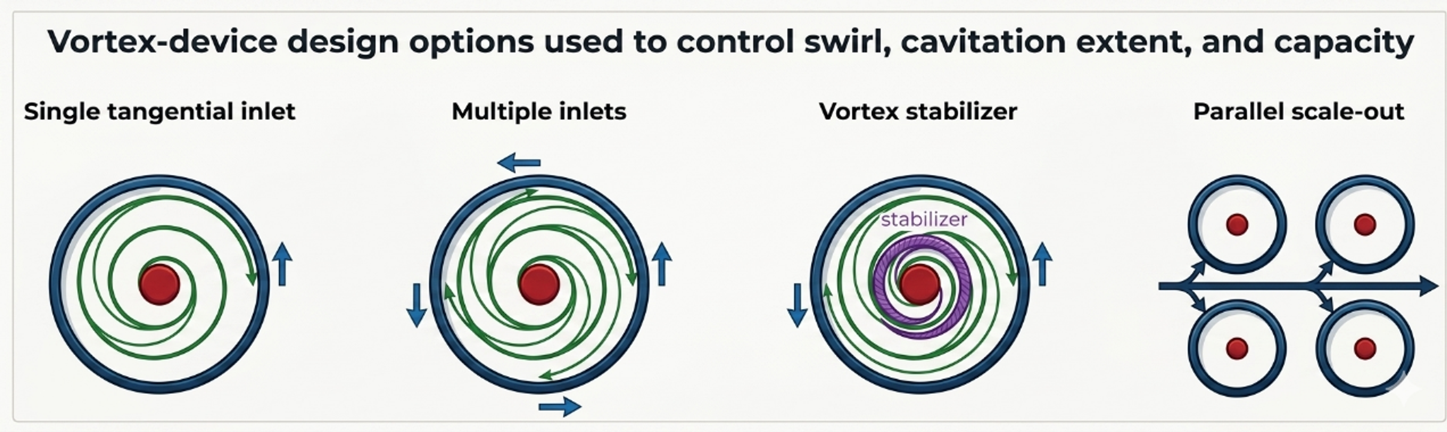
Figure 4.1. Representative vortex cavitation configurations and geometric variables [32].

4.1 Radial equilibrium screening model

For steady axisymmetric swirling flow with radial velocity small relative to tangential velocity, radial equilibrium is

where $V_{\theta }$ is tangential velocity and $r$ is radius from the axis. Outside a finite viscous core, an ideal free vortex can be represented as:

where $\mathrm{\Gamma }$ is circulation. Integrating Equation (4.1) between an outer radius $r_o$ at pressure $p_o$ and radius $r$ gives:

The mathematical free vortex predicts unbounded velocity and decreasing pressure as $r\to 0$, which is not physical. A preliminary device calculation therefore specifies a finite core radius $r_c$ and applies Equation (4.3) only for $r\ge r_c$. Inside the core, a forced vortex or measured profile is more appropriate.

The circulation required for the calculated pressure at $r_c$ to reach vapor pressure is:

Equation (4.4) is a useful screening criterion, but it does not predict the resulting vapor core radius. Once $p\le p_v$, a two phase core forms and modifies the velocity and pressure field. The criterion also depends strongly on the assumed $r_c$, which must be obtained from measurement, validated CFD, or a correlation for the selected chamber.

4.2 Tangential inlet and outlet sizing

For $N_i$ equal tangential inlets of area $A_i$, the nominal inlet velocity is:

The inlet Reynolds number should use the appropriate hydraulic diameter. Multiple inlets can improve azimuthal symmetry and distribute momentum, but their jets may interact differently as device scale, chamber aspect ratio, and inlet to chamber area ratio change.

A practical inlet velocity ratio is:

where $V_{\tan }$ and $V_{ax}$ are nominal tangential and axial velocity components at a defined station. $S_v$ is not the formal integral swirl number used in combustor analysis; it is a reproducible engineering ratio for a specific inlet geometry. When the inlet is purely tangential, the downstream axial component is generated by the outlet and internal recirculation, so it should be obtained from a mass balance or a resolved flow field.

The chamber aspect ratio is:

where $H_c$ is chamber height or axial length and $D_c$ is chamber diameter. Aspect ratio affects core residence, end wall interaction, and the distance available for vapor growth and recovery.

A vortex device Euler number based on inlet velocity is:

For a geometrically similar, calibrated vortex family, flow can be represented in the form:

where $K_v$ is an empirical capacity coefficient that contains inlet number, inlet ratio, outlet ratio, aspect ratio, and internal losses. Equation (4.9) is a family correlation, not a universal vortex law. Recent scale up studies demonstrate that device scale and geometry can change both cavitation and process response even when a global pressure drop parameter is preserved [7–10].

4.3 Outlet pressure, core stability, and recovery

The outlet must remove the required flow without suppressing the core or causing uncontrolled cavitation at an outlet edge. An undersized axial outlet increases backpressure and can shorten the vapor core; an oversized outlet may weaken the circulation or move recovery into downstream piping. An outlet tube extending into the chamber can stabilize or disturb the core depending on its diameter, insertion depth, and edge profile.

The following pressures should be distinguished:

• $p_o$, the pressure near the outer chamber radius used in a radial equilibrium model;

• $p_c$, the mean core pressure;

• $p_{out}$, the outlet pressure measured;

• $p_{\min }$, the instantaneous local minimum from a resolved model or high frequency measurement;

• $p_{rec}$, the pressure where cavity collapse is intended.

A vortex can continue to contain a gas rich or vapor rich core when the measured outlet pressure is well above vapor pressure. Conversely, low outlet pressure does not prove that the strongest collapse occurs inside the chamber. Imaging, pressure mapping, acoustic monitoring, and erosion inspection should be used together.

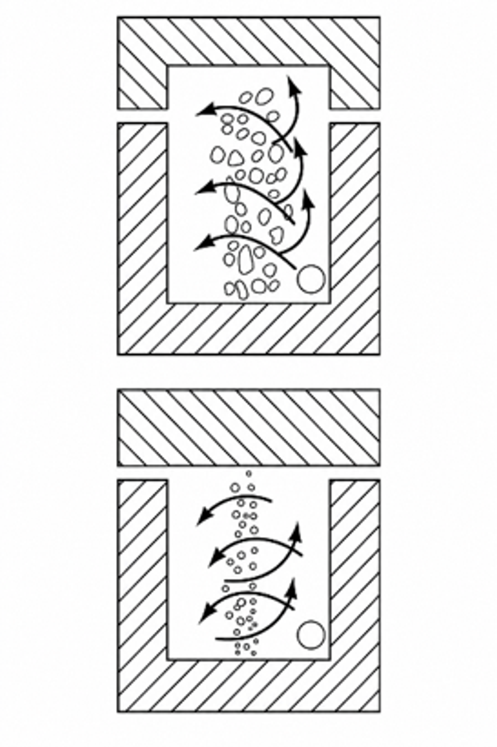
Figure 4.2. Vortex cavitation device showing tangential admission and axial core/outlet features. [14].

4.4 Worked Example 4.1: finite core vortex screen

Design basis. A water device at 25 °C has outer model radius $r_o=25$ mm, assumed finite core radius $r_c=4$ mm, and outer reference pressure $p_o=120$ kPa absolute. Four circular tangential inlets, each 4.0 mm in diameter, deliver $Q=3.0$ m³/h. Water properties are $\rho =997$ kg/m³ and $p_v=3.17$ kPa absolute. Circulation is varied to show the sensitivity of the single phase radial equilibrium model.

Equation (4.4) gives ${\mathrm{\Gamma }}_{crit}=0.390$ m²/s. Equation (4.3) gives the following core pressures:

Table 4.1. Worked Example 4.1 finite core results.

Circulation $𝚪$	Calculated $𝐩\left({𝐫}_{𝐜}\right)$ absolute	Interpretation
0.32 m²/s	41.3 kPa	Above vapor pressure in the single phase screen
0.36 m²/s	20.3 kPa	Strong pressure depression, but still above $p_v$
0.39 m²/s	3.04 kPa	Approximately the calculated inception boundary
0.42 m²/s	−15.7 kPa	Nonphysical single phase result; vapor core model is mandatory

Equation (4.5) gives a nominal velocity of 16.58 m/s in each of the four tangential inlets. The calculation does not determine the fraction of inlet momentum converted into circulation. That conversion depends on inlet orientation, wall friction, end wall flow, axial extraction, and turbulence. A measured velocity field or validated CFD is required to relate $V_i$ to $\mathrm{\Gamma }$.

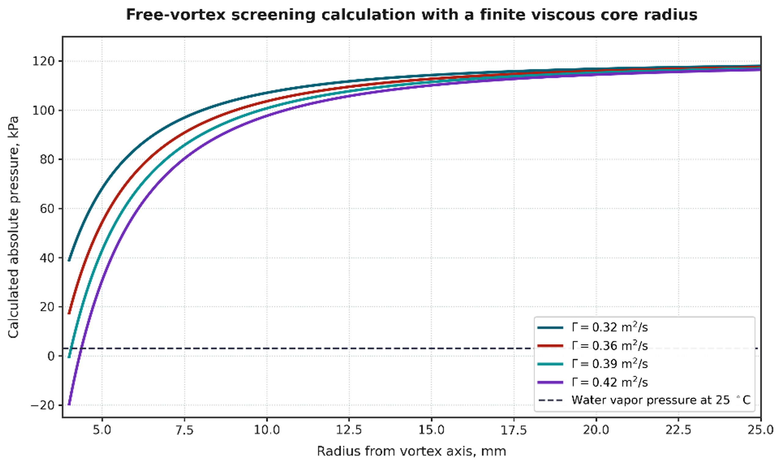
Figure 4.3. Calculated radial pressure profiles for Worked Example 4.1. Calculation using Equations (4.1) to (4.3). Where the single phase model predicts pressure below vapor pressure, a two phase cavitation model is required [32].

The worked example demonstrates two important design limits. First, the inferred core pressure is extremely sensitive to circulation and assumed core radius. Second, a negative absolute pressure from Equation (4.3) is not a prediction of a real negative pressure operating state. It indicates that the single phase model has crossed its validity boundary and must be replaced by a vapor core or multiphase model.

4.5 CFD and experimental calibration for vortex devices

A useful vortex CFD model should reproduce non cavitating pressure loss before cavitation parameters are adjusted. The mesh must resolve tangential inlets, near wall layers, outlet edges, and the core region. Transient simulation is often required because the core can precess and vapor clouds can shed. The selected cavitation model, nuclei density, bubble radius, mass transfer coefficients, turbulence model, and compressibility assumptions should be reported. Grid and time step independence should be demonstrated for pressure drop, core size, vapor volume, and dominant frequency, not only for a global residual [3, 4, 7].

Experimental calibration should include:

• a water flow pressure map at several backpressures;

• absolute pressure and temperature at every relevant station;

• visualization or a transparent development chamber where practicable;

• high frequency pressure or acoustic data to identify core precession and cloud shedding;

• flow distribution among parallel modules;

• product response versus pressure drop, passes, and scale;

• erosion or witness coupons at end walls, outlet edges, and recovery surfaces;

• repeat tests after dimensional wear to identify drift.

Studies of vortex devices for degradation and continuous emulsification show that pressure drop, number of passes, chamber geometry, device scale, dispersed phase fraction, and scale out arrangement affect performance. These results support the use of calibrated device families and parallel scale out rather than the assumption that one global cavitation number guarantees similarity [7–10].

4.6 Vortex scale up and scale out

For geometric scale up, inlet area, outlet area, chamber diameter, chamber height, and core stabilizer dimensions can be scaled by a common factor, but the absolute boundary layer thickness, viscous core, residence time, turbulence spectrum, and gas transport do not necessarily remain similar. Matching $E{u}_v$ and Reynolds number may require incompatible changes in flow and pressure. In addition, a larger chamber gives cavities more time to grow and can shift collapse toward an end wall or outlet.

Parallel scale out preserves the validated internal geometry. The manifold calculation should limit branch to branch flow variation, provide an isolation valve and pressure measurement for each module, and avoid a header pressure gradient that changes backpressure systematically across the array. The total capacity is:

where $N_m$ is number of modules. Uniformity can be reported as the coefficient of variation:

where $s_Q$ and $\bar{Q}$ are the standard deviation and mean of branch flows. The acceptable $C{V}_Q$ should be linked to the sensitivity of product performance to flow and pressure drop. A manifold that is hydraulically acceptable for ordinary heat exchange may still be too nonuniform for a narrow cavitation operating window.

Table 4.2. Vortex device calculation and validation checklist.

Item	Preliminary calculation	Calibration or acceptance evidence
Tangential inlets	Number, area, hydraulic diameter, velocity, $Re$, pressure loss	Measured branch or inlet flow and dimensional inspection
Chamber	$D_c$, $H_c$, $AR$, hold up, nominal residence time	Pressure map, visualization, residence time or tracer test
Core	$r_c$, ${\mathrm{\Gamma }}_{crit}$, calculated pressure profile	PIV, high speed imaging, CFD, acoustic or dynamic pressure signature
Outlet	Area ratio, velocity, insertion depth, recovered pressure	Stable flow pressure map and verified collapse location
Energy	$Q\mathrm{\Delta }p$, electrical input, heat balance	Calibrated electrical meter and temperature history
Scale up	$Re$, $E{u}_v$, geometry ratios, residence time	Pilot comparison at same product composition
Scale out	Header and branch losses, $C{V}_Q$, isolation	Individual branch flow or pressure confirmation
Integrity	End wall and outlet erosion screen	Coupons, thickness map, contamination analysis