Calculations of Hydrodynamic Cavitation Devices

3 Calculations for Static Hydrodynamic Cavitation Devices

Static hydrodynamic cavitation devices contain no moving cavitation generating element. Pump pressure energy is converted into local kinetic energy, separated flow, vortex motion, and irreversible pressure recovery. Principal calculation families include fixed restrictions such as orifices, nozzles, slit plates, and perforated inserts; Venturi and converging diverging passages; bluff bodies and jet impingement elements; and multistage combinations. Vortex chambers are mechanically static but are treated separately in Section 4 because their calculation method is distinct.

Static devices offer simple pressure containment, eliminate rotating seals, permit replaceable inserts, and integrate directly into pipelines. Their limitations include pump power demand, possible clogging, sensitivity to edge condition and fouling, and the possibility that attached cavities collapse near a wall. Static sizing should therefore determine both nominal hydraulic resistance and the intended locations of pressure depression and recovery [2–6].

3.1 Flow through orifice, nozzle, and slit devices

An orifice device divides the flow among one or more apertures. A sharp edged opening produces a contracted jet downstream of the physical aperture, and the minimum pressure commonly occurs near the vena contracta rather than at the downstream pressure tap. A rounded nozzle reduces separation and can shift inception and recovery. A slit provides a high perimeter to area ratio and can form a sheet like cavitation region, but it may be more sensitive to deformation, solids, and edge wear. Multi hole plates distribute flow among multiple jets and can increase the number of active regions; however, jet interaction, ligament thickness, plate thickness, and downstream chamber diameter become integral design variables [2,4–6].

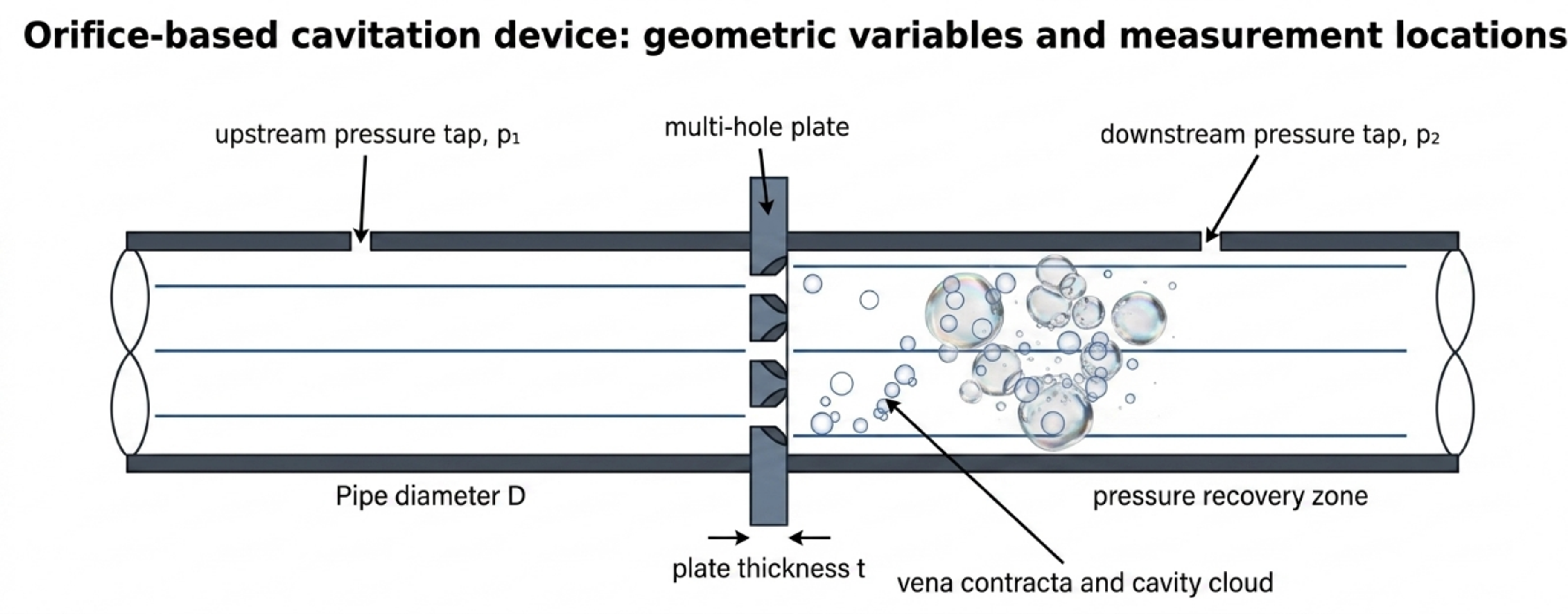
Figure 3.1. Flow through orifice geometry, principal dimensions, and pressure stations [32].

For an incompressible liquid, the basic calibrated relation is:

where $C_d$ is the discharge coefficient, $A_o$ is total open area, and $\mathrm{\Delta }p$ is the pressure difference associated with the stated measurement stations. Rearrangement gives the required total area:

For $N_h$ equal circular holes,

where $d_h$ is individual hole diameter. The nominal mean jet velocity based on the physical open area is:

and the hole Reynolds number is:

Two geometric ratios should be reported. The total open area fraction is:

where $A_p$ is pipe cross sectional area. The equivalent diameter ratio is:

where $D_p$ is pipe diameter and $d_{eq}$ is the diameter of one circular opening having the same total area. For a multi hole plate, ${\beta }_{eq}$ does not describe hole spacing, jet interaction, or minimum ligament. The individual ratio $d_h/D_p$ should also be reported.

The vena contracta area can be written $A_{vc}=C_c{A}_o$, where $C_c$ is the contraction coefficient. A one dimensional pressure screen is:

where $\mathrm{\Delta }{p}_{irr,1\to vc}$ represents irreversible loss accumulated before the vena contracta. Both $C_c$ and the local loss are geometry dependent. Equation (3.8) is useful for identifying whether the selected pressure drop can plausibly reach vapor pressure, but the result should not be presented as a measured minimum pressure unless it has been calibrated.

The pressure loss corresponding to the calibrated orifice relation is:

This quadratic dependence means that flow redistribution, fouling, edge damage, or partial blockage can change pressure drop sharply. A differential pressure alarm is therefore useful for both process control and condition monitoring.

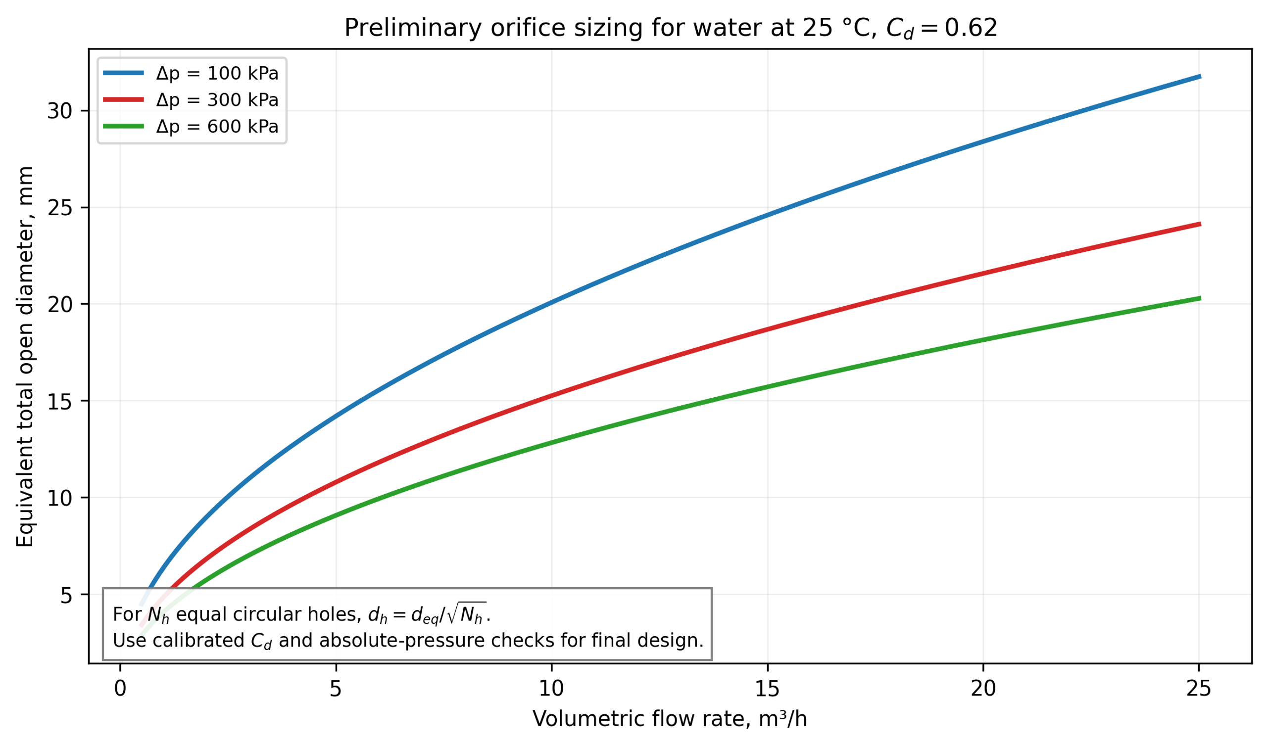
Figure 3.2. Equivalent total open diameter versus water flow for three pressure drops using a preliminary discharge coefficient C_d = 0.62 [32].

Selection and calibration of the discharge coefficient

The discharge coefficient is not a material constant. It represents contraction and energy loss and depends on Reynolds number, plate thickness to hole ratio, inlet edge radius, chamfer, hole shape, surface roughness, interaction among multiple holes, upstream velocity profile, and pressure tap arrangement. Standard differential pressure flow meter correlations such as ISO 5167 provide useful references for specified metering geometries, but a cavitating process insert may operate outside their validated geometry and flow regime [15, 16]. The recommended procedure is:

• Calculate a preliminary area using a conservative coefficient range.

• Fabricate a replaceable insert with measured dimensions and edge finish.

• Obtain a non cavitating water flow pressure curve over the intended Reynolds number range.

• Fit $C_d$ or a direct loss correlation using the exact pressure stations.

• Increase temperature or reduce backpressure to map cavitation inception and developed regimes.

• Repeat in the process fluid and check for viscosity, gas, solids, and rheology effects.

A pressure flow fit is more useful than a single coefficient because it reveals regime changes. If $C_d$ inferred from Equation (3.1) changes abruptly, the cause may be two phase choking, gas release, flow redistribution among holes, measurement dynamics, or a transition in the cavity structure.

Hole pattern and mechanical limits

A multi hole calculation must include more than total open area. Minimum hole diameter should be checked against the largest credible solid, fiber, agglomerate, crystal, or cleaning debris. The plate should retain adequate ligament between adjacent holes and between each hole and the outer sealing diameter. Plate bending, differential pressure, thermal shock, fatigue, and stress concentration around openings must be evaluated according to the applicable pressure code and fabrication standard. A thin sharp edge can produce a repeatable separated jet but is more susceptible to erosion and deformation; a thicker insert is mechanically stronger but alters the jet and may behave as a short tube.

For sanitary service, holes and downstream chambers must be inspectable and cleanable. A nominally self cleaning high velocity opening can still retain fibrous solids, crystallized salts, gums, or product in a low velocity recess. Hydraulic design should therefore be coordinated with drainability, clean in place velocity, gasket intrusion, and provision for a bypass or removable cartridge.

Table 3.1. Variables required to define a flow through restriction.

Variable	Symbol or description	Design significance
Pipe and chamber diameter	$D_p$, $D_c$	Upstream velocity, expansion ratio, recovery, jet interaction
Number and shape of openings	$N_h$; circular, slit, annular, conical	Distribution of jets, perimeter, blockage and cleanability
Opening dimension	$d_h$, slit width and length	Velocity, Reynolds number, minimum particle clearance
Total open area	$A_0$	Primary flow pressure sizing variable
Plate or insert thickness	$t_p$	Short tube behavior, strength, erosion path
Edge radius or chamfer	$r_e$ and angle	Separation and contraction coefficient
Hole pitch and ligament	$s_h$, $l_g$	Jet interaction, plate stress, manufacturability
Downstream standoff	$L_s$	Collapse location relative to wall, baffle, or next stage
Pressure tap locations	$L_{p1}$, $L_{p2}$	Reproducibility of $\mathrm{\Delta }p$, $C_d$, and $C_v$
Surface finish and material	roughness, alloy, coating	Inception, fouling, erosion, contamination

Worked Example 3.1: eight hole orifice plate

Design basis. Water at 25 °C is processed at $Q=5.00$ m³/h through a 40 mm internal diameter pipe. The selected measured pressure drop is 300 kPa. A preliminary discharge coefficient of 0.62 is used for sizing. The downstream reference pressure is absolute 150 kPa. Eight equal circular holes are selected. Water properties are $\rho =997$ kg/m³, $\mu =0.00089$ Pa·s, and $p_v=3.17$ kPa absolute.

Equation (3.2) gives:

$$A_o=9.13\times {10}^{-5}{m}^2$$

The equivalent single opening is 10.78 mm in diameter. Equation (3.3) gives an individual hole diameter of 3.81 mm. The nominal jet velocity from Equation (3.4) is 15.21 m/s, and Equation (3.5) gives $R{e}_o=6.50\times {10}^4$. The pipe area is $1.257\times {10}^{-3}$ m², so the total open area fraction is 0.0727. The ratio of each hole diameter to pipe diameter is 0.0953; the equivalent total diameter ratio is 0.2695.

The hydraulic power from Equation (2.12) is 416.7 W. If the aggregate pump, motor, and drive efficiency is 0.65, the assigned electrical input from Equation (2.13) is approximately 641 W. The single hydraulic energy pass from Equation (2.14) is 300.9 J/kg, equivalent to 0.0836 kWh per metric ton. Using downstream pressure and nominal jet velocity in Equation (2.8) gives $\sigma =1.27$. This value is only a defined operating index; the vena contracta pressure may be much lower than the downstream tap pressure.

Table 3.2. Worked Example 3.1 results.

Quantity	Value	Design interpretation
Flow rate	5.00 m³/h	Normal operating point; turndown and maximum flow also require checks
Measured pressure drop	300 kPa	Determines pump duty and calibrated flow relation
Total open area	91.3 mm²	Preliminary value using $C_d=0.62$
Number of holes	8	Must be coordinated with pitch and ligament
Individual hole diameter	3.81 mm	Verify solids clearance, tolerance, and erosion allowance
Nominal jet velocity	15.21 m/s	Physical area velocity, not vena contracta velocity
Hole Reynolds number	$6.50\times {10}^4$	Turbulent screening condition
Total open area fraction	7.27%	Strong contraction and downstream expansion
Hydraulic power	0.417 kW	Power transferred across the measured pressure drop
Estimated electrical power	0.641 kW	Uses aggregate efficiency 0.65; verify by measured input
Single pass hydraulic energy	300.9 J/kg	Does not specify the fraction delivered as useful collapse energy
Defined cavitation number	1.27	Based on $p_2=150$ kPa absolute and $V_j$; not directly comparable to other definitions

This example is a preliminary hydraulic size, not a final plate drawing. Final design requires the flow pressure curve, absolute inlet and outlet pressures, hole tolerance, edge profile, plate stress, gasket and flange details, pressure relief, minimum passage, and a cavitation map. The example also illustrates why a device can have modest total power yet a severe local pressure history

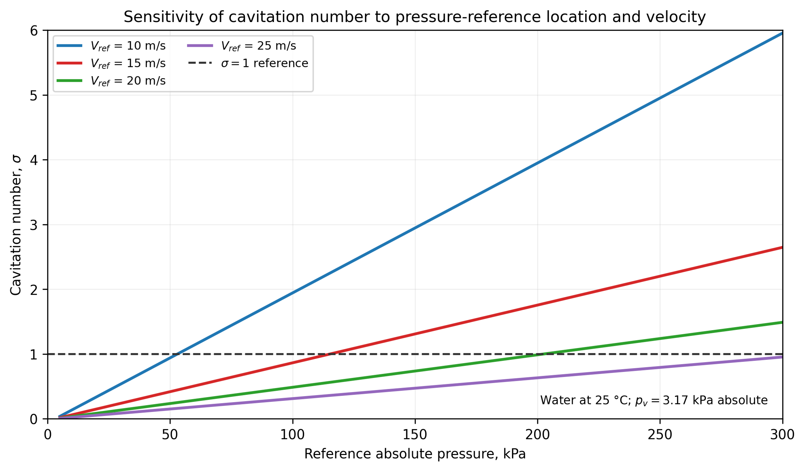
Figure 3.3. Sensitivity of the cavitation number to the selected absolute pressure and reference velocity for water at 25 °C [32].

3.2 Venturi based flow through devices

A Venturi cavitator consists of a converging section, a throat, and a diffuser. The calculation must define the contraction profile, throat diameter or hydraulic diameter, throat length, diffuser half angle, outlet diameter, surface finish, and pressure tap locations. Relative to a sharp orifice, a Venturi can provide a controlled low pressure residence interval and smoother recovery, although an aggressive diffuser can separate and generate an unsteady recovery field [4,6].

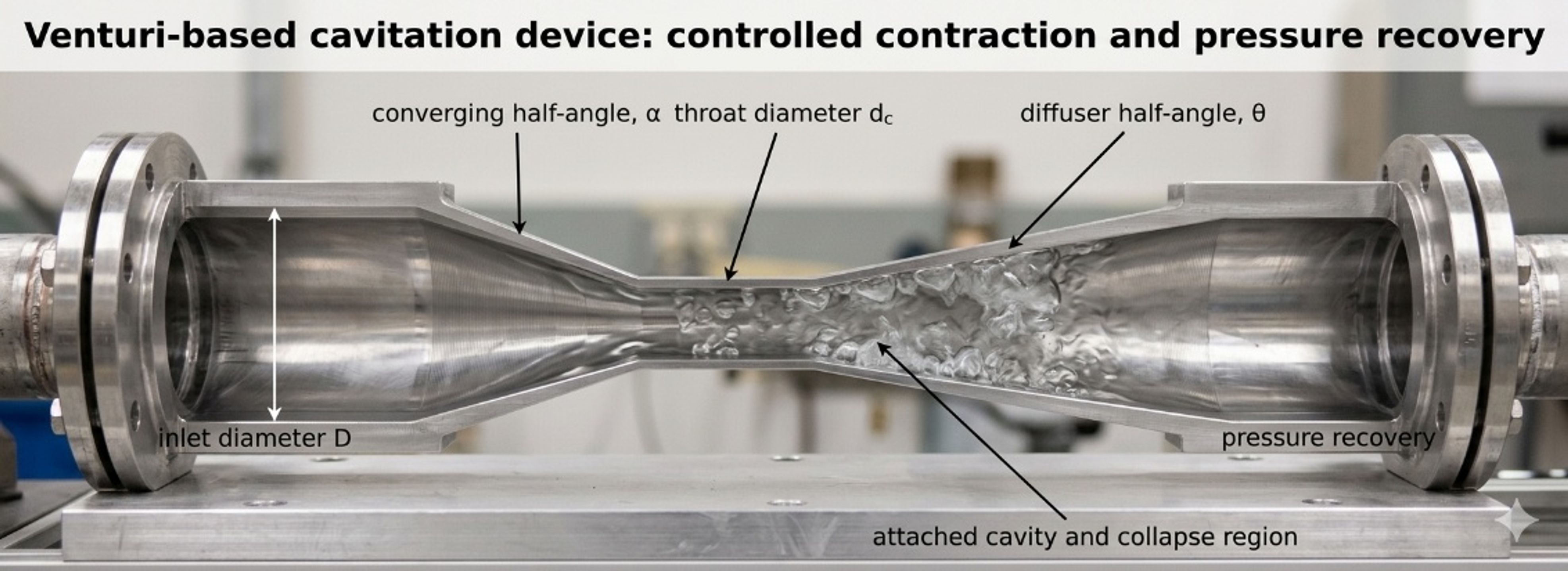
Figure 3.4. Venturi based cavitation element and principal geometric variables [32].

If the desired throat velocity is known, throat area is:

A loss free Bernoulli screen for the throat velocity is:

where $p_t$ is the selected throat pressure, usually near but not necessarily below $p_v$. This equation neglects contraction loss, wall friction, turbulence, vapor volume, and two phase choking. It therefore provides an ideal upper velocity or minimum area screen.

For a circular throat,

and the diameter ratio is:

For a calibrated incompressible Venturi relation,

where $\mathrm{\Delta }p$ is defined between the upstream and throat stations. The coefficient and tap arrangement must correspond to the actual geometry. Standard metering correlations should not be extrapolated automatically into developed cavitation or nonstandard diffuser geometries [15, 16].

Pressure recovery can be characterized by:

where $p_2$ is the downstream recovered pressure. A larger value indicates greater static pressure recovery for the defined stations, but the coefficient does not reveal local oscillation, separation, or erosion.

For a conical diffuser with half angle $\theta$,

where $D_2$ is the downstream diameter. Small angles require longer equipment but generally support more gradual recovery. Larger angles shorten the device but can increase separation. The optimum is geometry and Reynolds number dependent; final selection should use validated CFD or a measured recovery map [4,6].

For a noncircular throat, the hydraulic diameter is:

where $P_w$ is wetted perimeter. A slit Venturi may be sized using $D_h$ for Reynolds number and friction screens, but local corner flow, aspect ratio, and sidewall effects still require explicit treatment.

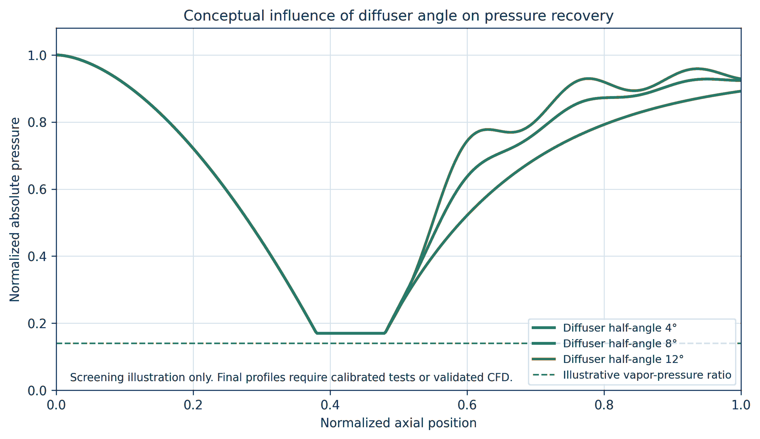
Figure 3.5. Conceptual effect of diffuser half angle on pressure recovery [32].

Worked Example 3.2: ideal throat screen

Design basis. Water at 25 °C flows at $Q=10.0$ m³/h through a 50 mm inlet. The inlet absolute pressure is 450 kPa. An ideal throat pressure target of 2.5 kPa absolute is used to screen the minimum throat area. This target is slightly below the equilibrium vapor pressure and intentionally signals that a single phase Bernoulli model has reached its limit.

The inlet velocity is 1.415 m/s. Equation (3.11) gives an ideal throat velocity of 30.0 m/s. Equations (3.10) and (3.12) give $A_t=9.26\times {10}^{-5}$ m² and $d_t=10.86$ mm. Equation (3.13) gives ${\beta }_t=0.217$.

For a return to 50 mm diameter, Equation (3.16) gives the following geometric lengths:

Table 3.3. Diffuser length screen for Worked Example 3.2.

Diffuser half angle	Calculated diffuser length
4°	0.280 m
6°	0.186 m
8°	0.139 m
10°	0.111 m
12°	0.092 m

The calculation does not imply that a 10.86 mm throat will maintain an absolute pressure of 2.5 kPa. Once vapor forms, the density field, momentum exchange, wall friction, compressibility, choking, and pressure recovery change. The calculated throat should therefore be treated as an initial geometry, followed by a realistic pressure profile obtained from a calibrated coefficient or CFD, sufficient throat length for the required cavity residence time, and testing of multiple diffuser geometries. Absolute inlet pressure must also be verified at minimum pump delivery and maximum operating temperature.

Venturi design checks

A final Venturi calculation should include:

• inlet and throat Reynolds numbers over the full viscosity range;

• contraction loss and the possibility of inlet separation;

• minimum absolute pressure and vapor fraction, not only inlet to outlet loss;

• throat residence time $L_t/V_t$;

• diffuser recovery and separation;

• downstream pressure needed to collapse cavities within a replaceable chamber;

• pressure pulsation and structural fatigue;

• throat wear, surface finish, and dimensional inspection;

• gas release and two phase choking;

• cleanability and minimum passage;

• pump curve, available suction head, and prevention of unintended pump cavitation.

3.3 Bluff body, wake, impingement, and multistage devices

A bluff body creates separated shear layers and a low pressure wake. Cavitation may form along the separation region, in periodic vortices, or where jets impinge and turn. The geometry can be a cone, cylinder, disk, wedge, baffle, liquid

whistle or opposed jet element. The global pressure drop can be represented by a loss coefficient, but useful calculation also requires blockage, wake length, shedding frequency, and the location of solid surfaces relative to collapse [2,4].

The blockage ratio is:

where $A_b$ is the projected bluff body area. Periodic wake behavior is characterized by the Strouhal number:

where $f_s$ is shedding frequency and $d_b$ is a characteristic body dimension. A measured acoustic peak should not be identified automatically as the shedding frequency because pump pulsation, structural resonance, cavity cloud oscillation, and blade or valve frequencies may overlap.

Multistage devices place several restrictions or baffles in series. The total measured loss is:

where $N_s$ is number of stages and $\mathrm{\Delta }{p}_{conn}$ includes connecting passages, expansions, and manifolds. The corresponding hydraulic power is:

Equal division of total pressure drop among stages is not guaranteed. Upstream gas release, temperature rise, changing vapor fraction, fouling, and different downstream recovery conditions can make nominally identical stages operate differently. Pressure measurements between stages or a validated model are required when stage by stage control is important.

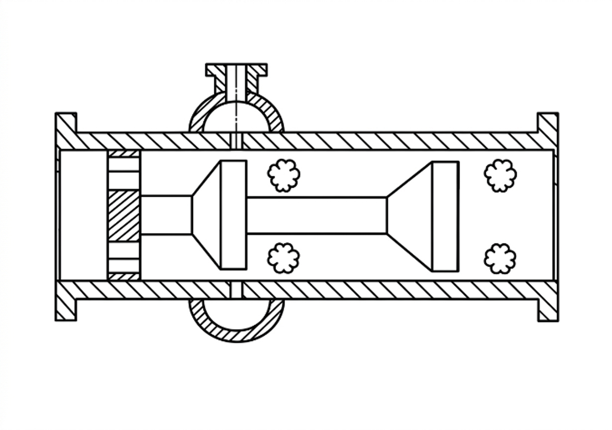
Figure 3.6. Multistage flow through cavitation device with repeated baffle elements. [13].

A multistage design should provide enough pressure recovery before the next restriction to obtain the intended collapse and regrowth sequence. If the pressure remains near vapor pressure throughout the device, the result may be a connected supercavity rather than repeated discrete collapse zones. Conversely, complete recovery at every stage can impose high cumulative pressure loss and concentrate erosion at each wall. Stage spacing, chamber diameter, baffle orientation, and intermediate pressure are therefore coupled with design variables.

Table 3.4. Calculation record for a multistage static device.

Stage	Restriction geometry	$𝐐$	${𝐩}_{𝐢𝐧}$ abs.	Estimated ${𝐩}_{\min }$ abs.	${𝐩}_{𝐨𝐮𝐭}$ abs.	$𝚫{𝐩}_{𝐢}$	Residence or spacing	Inspection feature
1	Hole, slit, cone, or baffle							Replaceable insert or coupon
2	Hole, slit, cone, or baffle							Intermediate tap
3	Hole, slit, cone, or baffle							Removable collapse chamber
$N_s$	Final element							Downstream thickness monitor

3.4 Static device scale up and scale out

Geometric enlargement of a static device changes absolute hole size, jet spacing, wall distance, residence time, pressure recovery, and the population of nuclei passing through each active zone. Keeping $\sigma$ constant does not preserve these quantities. A multi hole device can often be scaled by increasing the number of validated holes or by using parallel cartridges, but the manifold must distribute flow uniformly. A Venturi can be enlarged geometrically, but diffuser behavior and cavity length may not remain similar at a new Reynolds number and pressure scale. A bluff body device can change shedding and wake confinement as blockage and chamber dimensions change [4, 7–10].

The recommended scale up hierarchy is:

• Preserve the active geometric feature and its dimensionless ratios.

• Preserve the pressure history, including the recovery region, rather than only total pressure drop.

• Match the relevant Reynolds, Euler, Weber, and cavitation number definitions as closely as practical.

• Preserve or deliberately redesign the exposure time and number of active zones.

• Verify pressure, flow, cavity signature, product response, specific electrical energy, and material loss simultaneously.

• Prefer parallel scale out when one large device introduces a new, unvalidated flow structure.

A static device should be accepted only after the pump and piping system are considered. The cavitator may be correctly sized while the pump operates near suction cavitation, the downstream valve creates a second uncontrolled cavitation zone, or the recirculation line accumulates gas. The complete hydraulic system curve, pump curve, relief path, maximum blocked in pressure, and minimum downstream pressure belong in the calculation package.