Technical publication

Fundamentals

Single Cavitation Bubble Collapse: Phenomena, Theoretical Models, and Thermodynamic Effects

Dr. Oleg V. Kozyuk

okozyuk.com

Published September 29, 2026

Read complete publication for whole-document Find and printing. Browser Find and native printing on this reader include only loaded content.

3. Theoretical Models

3.1 Spherical Kinematics and the Pressure Field

The simplest derivation assumes a spherical bubble in an incompressible liquid of constant density. Conservation of liquid volume gives the radial velocity:

u (r, t) = \frac{R^{2} \dot{R}}{r^{2}}

[9]

A corresponding velocity potential is $ϕ = - R^{2} \dot{R} / r$ . Substitution into the unsteady Bernoulli equation gives the liquid pressure field:

p (r, t) - p_{\infty} (t) = ρ [\frac{R^{2} \ddot{R} + 2 R {\dot{R}}^{2}}{r} - \frac{R^{4} {\dot{R}}^{2}}{2 r^{4}}]

[10]

At the interface, $r = R$ , the pressure relation reduces to:

p_{L} - p_{\infty} = ρ (R \ddot{R} + \frac{3}{2} {\dot{R}}^{2})

[11]

where $p_{L}$ is the liquid pressure immediately outside the bubble. This relation is the inertial core of the Rayleigh and Rayleigh Plesset equations.

The assumptions are restrictive. Incompressibility implies instantaneous pressure communication and therefore cannot represent shock radiation. Spherical symmetry excludes jets, translation, and topology change. Even so, the formulation remains valuable because it isolates the balance among interface acceleration, convective inertia, and pressure.

3.2 Rayleigh Empty Cavity Model

Rayleigh considered an empty cavity for which vapor pressure is neglected relative to the external pressure [1]. More generally, define the constant collapse driving pressure as:

Δ p = p_{\infty} - p_{v} > 0

[12]

The radial equation is:

R \ddot{R} + \frac{3}{2} {\dot{R}}^{2} = - \frac{Δ p}{ρ}

[13]

Multiplication by $R^{2} \dot{R}$ and integration from the maximum radius, where $\dot{R} = 0$ , gives:

{\dot{R}}^{2} = \frac{2 Δ p}{3 ρ} [{(\frac{R_{\max}}{R})}^{3} - 1]

[14]

The wall speed therefore diverges as $R^{- 3 / 2}$ in the ideal model. A second integration gives the collapse time:

t_{R} = 0.914681 R_{\max} \sqrt{\frac{ρ}{Δ p}}

[15]

This relation is one of the most useful scaling laws in cavitation. It predicts that collapse time is proportional to bubble size, increases with liquid density, and decreases with the square root of the pressure difference. It is commonly used to normalize experimental time histories and to define a Rayleigh factor based on the ratio of measured collapse time to $R_{\max} \sqrt{ρ / Δ p}$ .

Figure 4. Dimensionless Rayleigh collapse trajectory obtained by numerical integration of the empty cavity equation . The ideal model reaches zero radius at the nominal collapse time with a divergent wall speed [1]Source reference: Rayleigh, Lord. On the Pressure Developed in a Liquid during the Collapse of a Spherical Cavity, 1917.

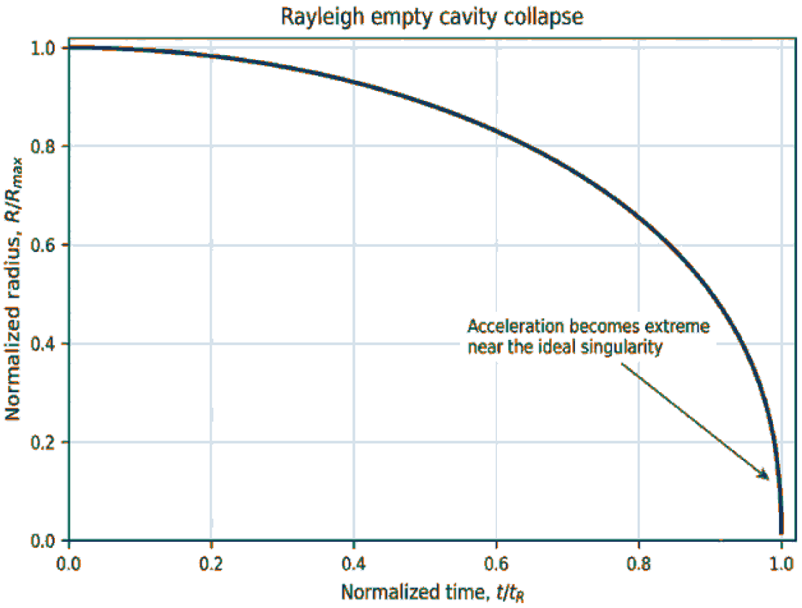
Figure 4. Dimensionless Rayleigh collapse trajectory obtained by numerical integration of the empty cavity equation [1]. The ideal model reaches zero radius at the nominal collapse time with a divergent wall speed.

The model predicts first order collapse time remarkably well for large vapor cavities when viscosity and surface tension are small and the bubble remains nearly spherical. It fails near the minimum radius, where compressibility and internal pressure dominate, and it cannot predict rebound, shock amplitude, or jet formation.

3.3 Rayleigh Plesset Equation

For a spherical bubble containing gas and vapor, the normal stress condition is:

p_{L} = p_{B} - \frac{2 γ}{R} - \frac{4 μ \dot{R}}{R}

[16]

Combining this condition with the inertial pressure balance gives the Rayleigh Plesset equation [2]:

R \ddot{R} + \frac{3}{2} {\dot{R}}^{2} = \frac{1}{ρ} [p_{B} (t) - p_{\infty} (t) - \frac{2 γ}{R} - \frac{4 μ \dot{R}}{R}]

[17]

An acoustically driven far field pressure can be represented as:

p_{\infty} (t) = p_{0} - p_{A} \sin (ω t)

[18]

where $p_{A}$ is the acoustic pressure amplitude. For a transient cavitation bubble, $p_{\infty} (t)$ can instead be specified as a pressure step, a measured waveform, or a computed local pressure history.

A common closure for the bubble pressure is:

p_{B} = p_{s a t} (T_{i}) + p_{g 0} {(\frac{R_{0}}{R})}^{3 κ}

[19]

with the equilibrium gas pressure:

p_{g 0} = p_{0} + \frac{2 γ}{R_{0}} - p_{s a t} (T_{\infty})

[20]

This closure treats vapor pressure as spatially uniform and permanent gas as polytropic. It is adequate for many moderate oscillations but becomes unreliable during violent collapse because $T_{i}$ and vapor mass change rapidly, the gas can become spatially nonuniform, and chemical reactions may occur [7,9,13,16].

Surface tension is most important for small bubbles, whereas viscosity becomes significant at small radii and lower Reynolds number. For a millimeter scale transient cavity in water, both effects are usually secondary through most of the first collapse but can become important near the minimum radius.

3.4 Interior Thermodynamic Closures

The principal uncertainty in a spherical bubble equation often lies not in liquid inertia but in the representation of $p_{B}$ . Several levels of thermodynamic closure are commonly used.

Constant vapor pressure and polytropic gas. This is the closure used above. The condition $κ = 1$ represents isothermal gas behavior, whereas $κ$ equal to the heat capacity ratio represents ideal adiabatic behavior. Real bubble oscillations generally lie between these limits, and the effective exponent depends on frequency and radius [7].

Uniform temperature energy model. The bubble contents are treated as well mixed. An energy equation determines the time dependent gas temperature, and the vapor mass changes through an interfacial flux. This formulation captures latent heat and variable pressure at moderate computational cost.

Radially resolved gas vapor model. Conservation equations for species, momentum or low Mach number flow, and energy are solved within the bubble. This approach resolves thermal boundary layers, vapor diffusion, nonequilibrium condensation, and chemical reactions [9,13,16]. It is required when accurate peak temperature or sonochemical predictions are needed.

Equation of state closure. At very high pressure, ideal gas behavior can become inadequate. A real gas equation of state and variable transport properties may be required. For cryogenic fluids or mixtures, phase equilibrium and fluid properties must be evaluated at the local composition and temperature [27,28].

The selected closure can materially change the predicted minimum radius, peak pressure, rebound energy, and radiated shock. Agreement with a measured radius history does not by itself establish that the internal temperature or composition is correct.

3.5 Keller Miksis Equation

The Rayleigh Plesset equation neglects the finite propagation speed of pressure disturbances. The Keller Miksis equation retains first order terms in the bubble wall Mach number $\dot{R} / c$ [8]. Its compact form is:

(1 - \frac{\dot{R}}{c}) R \ddot{R} + \frac{3}{2} (1 - \frac{\dot{R}}{3 c}) {\dot{R}}^{2} = \frac{1}{ρ} (1 + \frac{\dot{R}}{c} + \frac{R}{c} \frac{d}{d t}) [p_{L} - p_{\infty} (t)]

[21]

where:

p_{L} = p_{B} - \frac{2 γ}{R} - \frac{4 μ \dot{R}}{R}

[22]

The additional terms represent acoustic radiation and the delay associated with liquid compressibility. The equation is widely used because it is only modestly more expensive to integrate than Rayleigh Plesset while providing more realistic damping and collapse pressure when $| \dot{R} | / c$ remains moderate. It becomes less reliable as the wall Mach number approaches unity or when the liquid equation of state becomes strongly nonlinear.

A practical advantage is that measured or prescribed acoustic pressure waveforms can be introduced directly. A practical limitation is numerical stiffness near collapse. The internal pressure model and its time derivative must also be implemented consistently. Discontinuous forcing or an overly crude vapor pressure closure can generate unphysical pressure spikes.

3.6 Gilmore Equation

Gilmore formulated spherical bubble dynamics in terms of the enthalpy and local sound speed of a compressible liquid [3]. The governing equation is:

(1 - \frac{\dot{R}}{C}) R \ddot{R} + \frac{3}{2} (1 - \frac{\dot{R}}{3 C}) {\dot{R}}^{2} = (1 + \frac{\dot{R}}{C}) H + (1 - \frac{\dot{R}}{C}) \frac{R}{C} \dot{H}

[23]

where:

H = \int_{p_{\infty}}^{p_{L}} \frac{d p}{ρ (p)}

[24]

$C$ is the liquid enthalpy difference, and $ρ (p)$ is the sound speed evaluated at the liquid pressure adjacent to the wall. A liquid equation of state, commonly a Tait type relation for water, supplies the required relations for $ρ (p)$ and density as functions of pressure.

The Gilmore equation is preferred when the pressure near the bubble wall is sufficiently high that sound speed and density differ substantially from their ambient values. It can represent strong compression and shock emission more robustly than a constant sound speed equation. It remains a spherical model and cannot resolve the propagated shock profile after the wave leaves the bubble. Far field pressure must therefore be obtained from an acoustic propagation relation or a separate compressible flow calculation.

Prosperetti and Lezzi derived a systematic family of compressible bubble equations by expansion in a small Mach number parameter [10,11]. The first order theory contains a free parameter that recovers several earlier formulations for particular choices, while the second order theory retains additional compressibility terms. This analysis is important because it distinguishes approximations that are formally equivalent to first order from differences that become significant at the next order.

In practical calculations, selection among Keller Miksis, Gilmore, and Prosperetti Lezzi formulations should be based on the pressure range, expected wall Mach number, and required output. First order equations are often sufficient for radius histories and moderate acoustic radiation. Very high pressures favor a variable property formulation or direct compressible simulation. No radial equation can predict a wall directed microjet.

3.8 Nonequilibrium Condensation and Phase Change Models

Fujikawa and Akamatsu showed that nonequilibrium condensation can alter the pressure wave generated by bubble collapse [9]. In a pure vapor cavity, instantaneous equilibrium would impose $p_{v} = p_{s a t} (T_{i})$ at every instant. In reality, condensation is limited by molecular accommodation, diffusion, and heat removal. Vapor can therefore remain supersaturated or undergo substantial compression before condensation.

A simplified kinetic relation for the interfacial vapor mass flux is the Hertz Knudsen form:

j = α_{m} \frac{p_{s a t} (T_{i}) - p_{v}}{\sqrt{2 π R_{v} T_{i}}}

[25]

where $α_{m}$ is the mass accommodation coefficient and $R_{v}$ is the specific gas constant of the vapor. Positive $j$ denotes net evaporation into the bubble. The relation is useful as a closure, although $α_{m}$ is often treated as an effective parameter because interface kinetics, contamination, and temperature nonuniformity are not fully resolved.

Phase change models become especially important for high vapor pressure liquids, hot water, cryogenic propellants, and mixtures. Under these conditions, vapor mass is not merely a passive pressure offset. It acts as a dynamic reservoir of energy and momentum.

3.9 Nonspherical Potential Flow and Boundary Integral Models

When viscosity and vorticity are confined to thin regions, the external liquid can be approximated as potential flow:

\nabla^{2} ϕ = 0

[26]

The bubble surface moves with the liquid according to:

\frac{D x}{D t} = \nabla ϕ

[27]

The velocity potential on the interface satisfies:

\frac{D ϕ}{D t} = \frac{1}{2} | \nabla ϕ |^{2} + \frac{p_{\infty} - p_{L}}{ρ}

[28]

A boundary integral formulation converts the Laplace problem into an integral over the bubble and solid boundaries. Only the surfaces require discretization, making the method efficient for large interface deformation. Image systems or explicit boundary panels can enforce rigid wall or free surface conditions. Weak compressibility corrections can also be introduced, as in the formulations of Wang and Blake [19,21].

Boundary integral methods predict migration, jet formation, toroidal transition, and the dependence of jet direction on the forcing field. Their principal limitations arise from the assumptions of irrotational flow and a single valued interface representation. Jet impact creates a topological change that requires special reconnection algorithms. After impact, vortex rings, splashing, and fragmentation become increasingly important, while strong shock propagation lies outside the scope of incompressible potential flow.

3.10 Compressible Multiphase Computational Fluid Dynamics

Direct numerical simulation solves conservation equations in both phases or within a mixture formulation. Interface capturing methods such as volume of fluid, level set, and diffuse interface schemes can represent jet impact, toroidal bubbles, breakup, and shock interaction. A general compressible two phase formulation includes:

\frac{\partial ρ}{\partial t} + \nabla \cdot (ρ u) = 0

[29]

\frac{\partial (ρ u)}{\partial t} + \nabla \cdot (ρ u u + p I - τ) = ρ g + f_{γ}

[30]

and:

\frac{\partial (ρ E)}{\partial t} + \nabla \cdot [(ρ E + p) u - τ \cdot u + q] = {\dot{Q}}_{p h a s e}

[31]

The equation of state, interface method, surface tension treatment, and phase change source terms determine the physical fidelity of the calculation. The computational challenge is severe because the bubble radius, thermal boundary layer, jet tip, and shock thickness occupy very different length scales. Numerical diffusion can smear the interface and reduce peak pressure, whereas insufficient spatial resolution can delay jet impact or alter fragmentation.

Compressible multiphase computational fluid dynamics is most appropriate when the research question concerns shock structure, topology change, interaction with complex geometry, or local wall loading. Validation should include radius history, jet velocity, shock arrival time, and energy conservation rather than a single output alone.

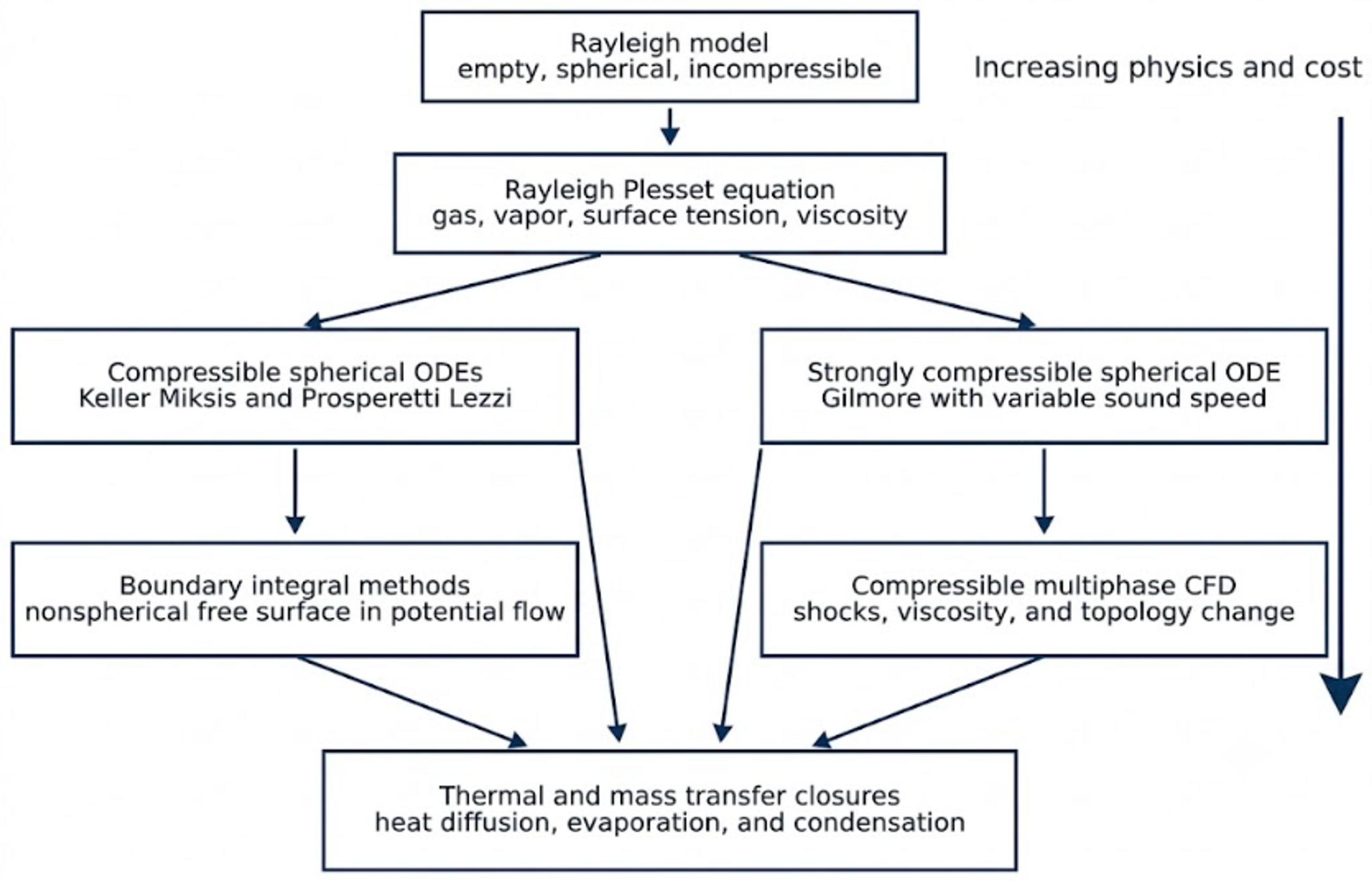
Figure 5. Hierarchy of common single bubble models. Increasing physical completeness generally requires increasing computational cost. [32]

3.11 Dimensionless Groups and Model Selection

Using the characteristic velocity $U_{R} = \sqrt{Δ p / ρ}$ and characteristic length $R_{\max}$ , the following dimensionless groups indicate the relative importance of the principal physical mechanisms.

Table 2. Dimensionless groups for single bubble dynamics.

Group	Definition	Physical interpretation
Mach number	$M a = U_{R} / c$ or $\| \dot{R} \| / c$	Importance of liquid compressibility and shock formation
Reynolds number	$R e = ρ R_{\max} U_{R} / μ$	Ratio of inertia to viscosity
Weber number	$W e = ρ R_{\max} U_{R}^{2} / γ$	Ratio of inertia to surface tension
Thermal Peclet number	$P e_{T} = R_{\max} U_{R} / α_{l}$	Ratio of advection time to thermal diffusion time
Fourier number	$F o = α_{l} t / R_{\max}^{2}$	Fraction of the radius reached by thermal diffusion
Jakob number	$J a = ρ_{l} c_{p, l} \| T_{\infty} - T_{i} \| / (ρ_{v} L)$	Sensible heat available relative to latent heat demand
Standoff parameter	$γ_{s} = h / R_{\max}$	Strength of a nearby wall influence
Anisotropy parameter	$ζ = \| \nabla p \| R_{\max} / Δ p$	Normalized pressure gradient or Kelvin impulse scale

A practical model selection sequence is as follows:

Use the Rayleigh model for an initial estimate of collapse time and characteristic velocity.
Use Rayleigh Plesset for spherical motion when liquid compressibility is weak and shock amplitude is not required.
Use Keller Miksis or a first order Prosperetti Lezzi equation when acoustic radiation and moderate wall Mach number are important.
Use Gilmore when liquid properties vary strongly with pressure or when the collapse is very violent.
Use a boundary integral method for nonspherical deformation and jetting when shocks and viscosity are secondary.
Use compressible multiphase computational fluid dynamics when shocks, jets, topology change, and complex boundary interactions must be resolved simultaneously.
Add coupled heat and mass transfer whenever vapor pressure, condensation rate, or peak temperature is central to the analysis.

Table 3. Comparison of principal theoretical models.

Model	Included physics	Best use	Main limitation
Rayleigh [1]	Spherical inertia and constant pressure difference	Collapse time and scaling	Empty cavity, no rebound, no shock physics
Rayleigh Plesset [2]	Gas pressure, vapor pressure, surface tension, viscosity	Moderate spherical oscillations	Incompressible liquid
Keller Miksis [8]	First order liquid compressibility	Acoustic driving and radiative damping	Constant reference sound speed, spherical shape
Gilmore [3]	Variable density, sound speed, and enthalpy	Strong spherical collapse	Requires liquid equation of state, no jets
Prosperetti Lezzi [10,11]	Systematic first and second order compressibility	Error controlled radial modeling	More complex implementation
Boundary integral [19,21]	Nonspherical potential flow and boundaries	Migration, jetting, topology studies	Weak shock and viscous capability
Compressible multiphase CFD	Shocks, viscosity, complex geometry, topology change	Local loads and coupled flow structure	High computational cost and resolution sensitivity
Thermal phase change model [9,13,16]	Heat transfer, vapor transport, reactions	Vapor rich, hot, cryogenic, or luminous collapse	Property data and closure uncertainty