Technical publication

Reactors & equipment

Hydrodynamic Cavitation in Emulsification and Homogenization

Dr. Oleg V. Kozyuk

okozyuk.com

Published October 1, 2026

Read complete publication for whole-document Find and printing. Browser Find and native printing on this reader include only loaded content.

4 Mathematical Models of Cavitation Assisted Emulsification

4.1 Modeling hierarchy and required data

No single model captures all scales from pump and piping hydraulics to nanometre scale interface rupture. A practical hierarchy begins with hydraulic calculations, adds a specific device description, applies a droplet breakup and coalescence model, and closes the calculation with surfactant adsorption and product rheology. The model should be chosen according to the available measurements and design question. A correlation may be adequate for selecting pressure and pass number in an established device. New geometry and scale up generally require computational fluid dynamics coupled to population balances or a validated reduced order model [19,24–29].

Table 4. Model hierarchy for hydrodynamic cavitation emulsification.

Model level	Main outputs	Required inputs	Appropriate use	Main limitation
Hydraulic balance	Flow, pressure drop, residence time, energy	Geometry, pump curve, fluid properties	Preliminary sizing and utility estimate	No droplet prediction
Dimensionless correlation	Cavitation number, Weber number, expected diameter trend	Pressure, velocity, interfacial tension, density	Operating window screening	Device specific constants
Kolmogorov and Hinze model	Maximum stable diameter	Local energy dissipation and interfacial properties	Turbulent breakup estimate	Cannot represent collapse intermittency directly
Bubble field model	Droplet size from bubble diameter, concentration, and collapse pressure	Bubble statistics, pressure, interfacial tension	Controlled flow cavitation design	Strong simplifying assumptions and difficult bubble measurements
Population balance model	Full droplet size distribution	Flow field, breakup and coalescence kernels	Geometry evaluation and distribution prediction	Calibration and computational cost
Reduced three population model	Fast approximation of multimodal DSD evolution	Rate constants correlated with energy and composition	Control, scale up screening, digital twin	Coarse representation of the distribution
Empirical response surface	Optimum conditions in a tested range	Designed experimental data	Formulation optimization	Poor extrapolation outside the design space

4.2 Kozyuk and Fedotkin bubble field model

The proposed mathematical model describes flow in cavitation mixers using established approaches to mixing processes and isotropic turbulence [21,22,30]. Its purpose is to relate the maximum stable emulsion droplet size to measurable characteristics of the collapsing bubble field. The model is based on the Kolmogorov and Hinze relation, expressed using the notation adopted in this article:

d_{k,max} \approx 3.5 {(\frac{γ}{ρ})}^{0.6} ε^{- 0.4}

[30]

The central model assumption is that the effective dissipation responsible for breakup is the dissipation associated with cavitation collapse:

ε = ε_{k}

[31]

Therefore,

d_{k,max} \approx 3.5 {(\frac{γ}{ρ})}^{0.6} ε_{k}^{- 0.4}

[32]

The rate associated with a single bubble of initial diameter $D_{0}$ is represented as:

ε_{k}^{b} (D_{0}) = \frac{E_{k}^{b}}{t} = \frac{π P D_{0}^{3}}{6 t}

[33]

where $P$ is the pressure surrounding the cavity during collapse and $t$ is collapse time. For a field of bubbles with size distribution $f (D_{0})$ , the total rate is averaged as:

ε_{k} = \int_{0}^{\infty} ε_{k}^{b} (D_{0}) f (D_{0}) d D_{0}

[34]

The model approximates the number distribution by a normal form whose integral equals the number of bubbles collapsing per unit mass, $n$ :

f (D_{0}) = \frac{n}{\sqrt{2 π} s_{D}} exp [- \frac{{(D_{0} - D_{m})}^{2}}{2 s_{D}^{2}}]

[35]

where $D_{m}$ is the mean bubble diameter and $s_{D}$ is the distribution standard deviation. Substitution gives:

ε_{k} = 1.18 \times 10^{- 1} \frac{\sqrt{π} Pn}{s_{D} t} I_{3} (D_{m}, s_{D})

[36]

with the third moment integral:

I_{3} (D_{m}, s_{D}) = \int_{0}^{\infty} D_{0}^{3} exp [- \frac{{(D_{0} - D_{m})}^{2}}{2 s_{D}^{2}}] d D_{0}

[37]

Using a parabolic cylinder function representation,

I_{3} = s_{D}^{4} exp (- \frac{D_{m}^{2}}{4 s_{D}^{2}}) Γ (4) D_{- 4} (- \frac{D_{m}}{s_{D}})

[38]

The Rayleigh collapse time based on the mean diameter is:

t = 0.91468 R_{m} \sqrt{\frac{ρ}{P}} = 0.45734 D_{m} \sqrt{\frac{ρ}{P}}

[39]

After substitution and simplification, the collapse field dissipation becomes:

ε_{k} = 2.74 \frac{P^{3 / 2} s_{D}^{3} n}{D_{m} \sqrt{ρ}} exp (- \frac{D_{m}^{2}}{4 s_{D}^{2}}) D_{- 4} (- \frac{D_{m}}{s_{D}})

[40]

To write the final droplet relation compactly, define a distribution factor:

F_{D} =exp (\frac{D_{m}^{2}}{10 s_{D}^{2}}) D_{m}^{0.4} s_{D}^{- 1.2} {[D_{- 4} (- \frac{D_{m}}{s_{D}})]}^{- 0.4}

[41]

The maximum stable droplet diameter may then be expressed as:

d_{k,max} = 2.34 {(\frac{γ}{P})}^{0.6} {(ρ n)}^{- 0.4} F_{D}

[42]

If bubbles are convected with the liquid and $N$ is the number concentration per unit liquid volume, the number per unit mass is:

n = \frac{N}{ρ}

[43]

which gives the final form:

d_{k,max} = 2.34 {(\frac{γ}{P})}^{0.6} N^{- 0.4} F_{D}

[44]

Equations (30) through (44) are useful because they make the design hypothesis explicit: smaller stable droplets are favored by lower interfacial tension, higher collapse pressure, a larger concentration of collapsing bubbles, and a bubble distribution that produces a favorable high order moment. The model also makes clear what must be measured: $D_{m}$ , $s_{D}$ , $N$ , $P$ , and $γ$ .

The model should be used with several qualifications. The normal distribution is not truncated mathematically and therefore permits negative diameters in principle, although the approximation is acceptable when $D_{m} / s_{D}$ is sufficiently large. A lognormal or gamma distribution is often more physical. The derivation assigns collapse energy to breakup without an explicit efficiency factor and does not include heat, sound, chemical reactions, wall effects, shielding among bubbles, or the probability that a droplet is close enough to a collapse event. The use of Kolmogorov and Hinze scaling assumes a turbulence like stress balance even though collapse is intermittent. Consequently, Equation (44) is best treated as a physically motivated engineering model that requires calibration against bubble visualization and droplet size measurements for each device family.

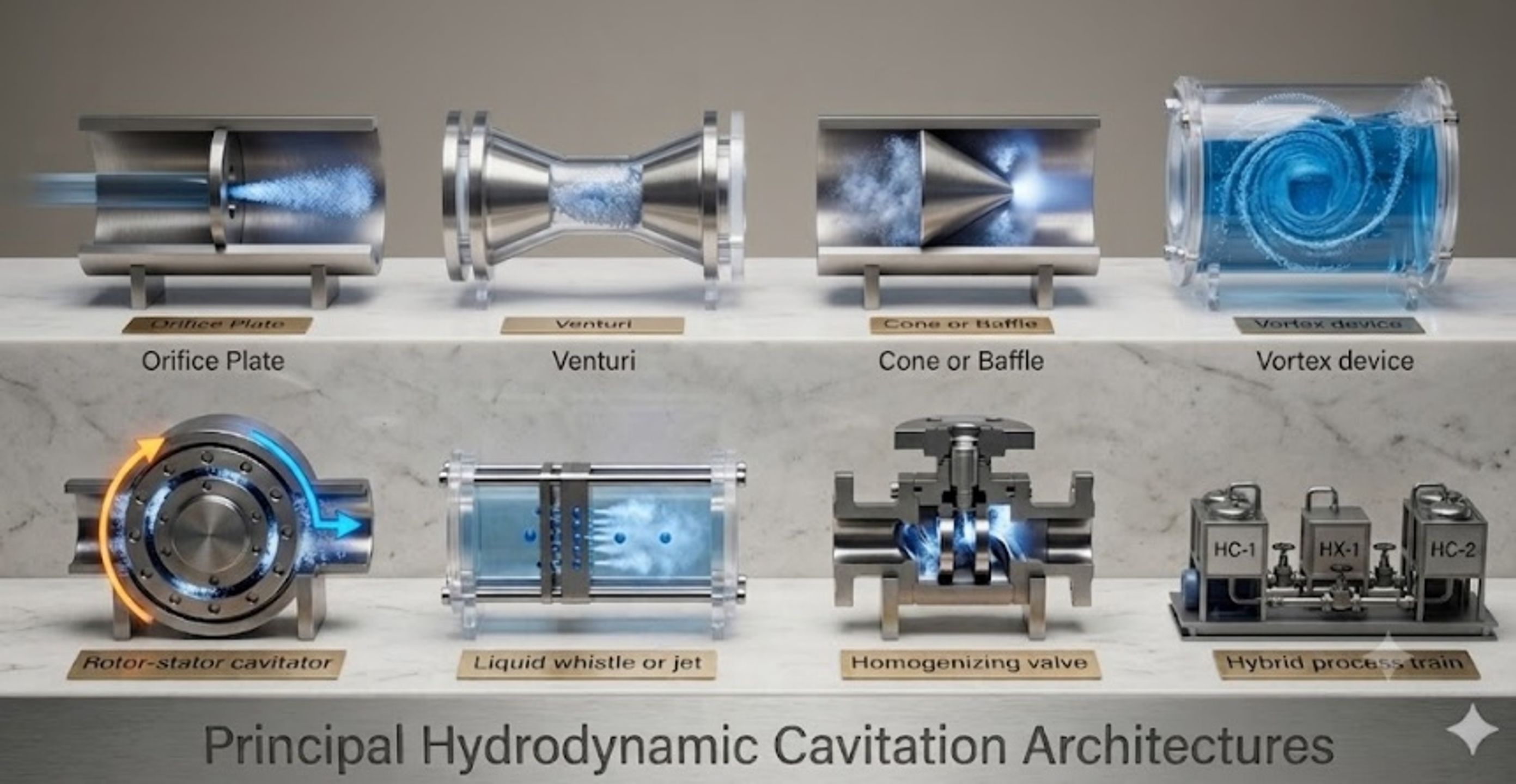
Figure 5. Principal hydrodynamic cavitation architectures used for emulsification and homogenization, including orifice, Venturi, cone or baffle, vortex, liquid whistle, and rotor stator devices [9].

Table 5. Assumptions and validation requirements for the Kozyuk and Fedotkin bubble field model.

Assumption	Engineering meaning	Likely effect if violated	Recommended validation
Breakup follows isotropic turbulence scaling	Collapse energy is mapped to a Hinze type stress balance	Device specific intermittency may be underrepresented	Compare predicted $d_{max}$ with measured $d_{90}$ over pressure and passes
Collapse energy dominates effective dissipation	Ordinary shear and extension are secondary	Model may overattribute breakup to cavitation	Run noncavitating pressure drop controls at similar flow
Bubble diameters follow a normal distribution	Two parameters describe the bubble field	Skewed and multimodal clouds may change high moments	High speed imaging or optical probes; test lognormal and gamma forms
All bubbles are convected with zero slip	Number per mass is $N / ρ$	Buoyancy, coalescence, and gas accumulation alter exposure	Measure void fraction and bubble velocity in the active zone
A representative collapse pressure exists	One $P$ characterizes recovery	Spatial and temporal pressure fluctuations are reduced to one value	Fast pressure transducers and CFD pressure histories
Droplet stabilization is instantaneous	Predicted breakup is retained	Recoalescence increases final diameter	Measure adsorption time, surfactant concentration, and post device aging

4.3 Population balance and reduced order models

A population balance represents the number density $n (v, x, t)$ of droplets with volume $v$ at position $x$ and time $t$ . A general transport equation is:

\frac{∂ n}{∂ t} + ∇⋅ (u n) = B_{br} - D_{br} + B_{co} - D_{co}

[45]

where the right hand terms are birth and death by breakup and coalescence. Breakup daughter distributions must conserve dispersed phase volume:

\int_{0}^{v_{p}} v b (v | v_{p}) d v = v_{p}

[46]

A generic breakup frequency can be written:

S (v, x) = C_{b} ε {(x)}^{a} v^{b} F (We, Oh, λ, C_{v})

[47]

where the exponents and function $F$ are calibrated to the selected physical model and device. Coalescence is commonly decomposed into collision and film drainage contributions:

K_{co} (v_{i}, v_{j}) = β_{coll} (v_{i}, v_{j}) P_{coal} (v_{i}, v_{j})

[48]

Full CFD and population balance calculations can represent spatially varying turbulence, vapor fraction, pressure, residence time, and emulsion rheology, but they remain sensitive to the cavitation model and breakup kernel. Open access numerical studies of cavitating devices and emulsion handling equipment show how geometry, vapor fraction, rheology, and dispersed phase distributions can be connected, although breakup closures remain formulation specific [19,31,32]. Recent open access single drop and turbulence studies provide complementary information for selecting breakup sub models [25–27].

A reduced model can represent the distribution by three droplet populations associated with low, medium, and intense stress zones. The following compact equations are an engineering representation inspired by open access reviews of stochastic breakup and by reduced order continuous emulsification modeling [27,28]:

\frac{d α_{1}}{d t} =- k_{12} α_{1} - k_{13} α_{1} - k_{1} (α_{1} - α_{1,min})

[49]

\frac{d α_{2}}{d t} = k_{12} α_{1} - k_{23} α_{2} - k_{2} (α_{2} - α_{2,min})

[50]

\frac{d α_{3}}{d t} = k_{13} α_{1} + k_{23} α_{2}

[51]

where $α_{j}$ is dispersed phase volume fraction in population $j$ and $k_{ji}$ are transfer rates caused by breakup. A volume fraction weighted Sauter mean can be reconstructed from representative diameters $d_{j}$ :

d_{32} = \frac{\sum_{j}^{} α_{j}}{\sum_{j}^{} α_{j} / d_{j}}

[52]

This representation preserves interpretability and is fast enough for optimization or control. It does not replace a full PBM when a detailed continuous distribution, coalescence, or multimodal daughter distribution is required.

Experiments with dense rapeseed oil emulsions in a vortex cavitation device found that the Sauter mean diameter decreased approximately with pass number as [24]:

d_{32} = K_{n} n_{p}^{- 0.2}

[53]

and the reported droplet breakage efficiency decreased with specific energy as:

η_{b} = K_{E} E^{- 0.8}

[54]

The negative energy exponent reflects diminishing returns: the largest droplets are disrupted first, while further reduction requires increasingly rare or intense events. The constants are formulation and device specific and should not be transferred without validation.

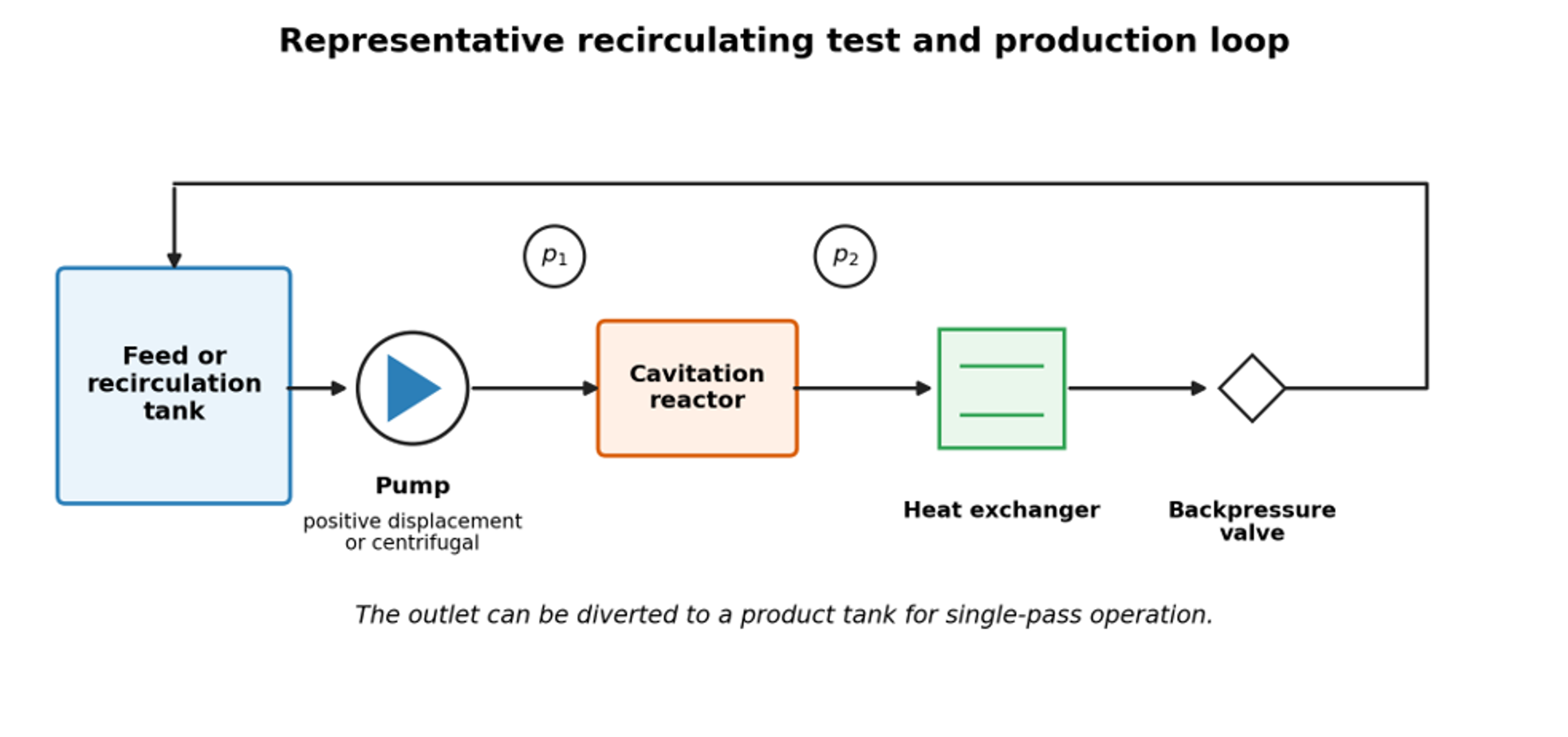
Figure 6. Representative recirculating test and production loop. Backpressure controls the recovery field; the same loop can be operated in recirculation or single pass mode [9].

4.4 Interfacial stabilization and recoalescence

The minimum surfactant mass needed to cover a newly created area $A$ is:

m_{s,min} = Γ_{\infty} A

[55]

where $Γ_{\infty}$ is the saturated surface excess. Coverage kinetics may be approximated by:

\frac{d θ}{d t} = k_{a} C_{s} (1 - θ) - k_{d} θ

[56]

where $θ$ is fractional coverage, $k_{a}$ and $k_{d}$ are adsorption and desorption coefficients, and $C_{s}$ is surfactant concentration in the continuous phase. A useful stabilization ratio is:

D a_{ads} = \frac{t_{exp}}{t_{ads}}

[57]

where $t_{exp}$ is the time between interface creation and a significant collision or exit from the active zone, and $t_{ads}$ is the characteristic adsorption time. When $D a_{ads} ≫ 1$ , coverage is comparatively fast. When $D a_{ads} ≪ 1$ , breakup may be followed by rapid recoalescence. Proteins and polymers often adsorb more slowly than small molecule surfactants, so identical cavitation conditions can produce different final sizes even at similar equilibrium interfacial tension.

For process comparison, net interface generated per specific energy can be written as:

A_{E} = \frac{a_{v,out} - a_{v,in}}{E_{in}}

[58]

and a thermodynamic emulsification efficiency can be defined as:

η_{th} = \frac{γ (A_{out} - A_{in})}{E_{in}}

[59]

A useful comparison therefore reports the product droplet size distribution, newly generated interface, hydraulic work, electrical energy, temperature rise, and pass count together. Open access studies emphasize that the local breakup field and mixing configuration, not nominal power alone, determine the useful outcome [12,13,26,27].

4.5 Worked engineering example: model based hydraulic and interfacial screening

For an illustrative screening calculation, assume a 3 mm circular throat carrying 13.6 L/min of a water continuous premix across a 1.0 MPa pressure drop. These values are hypothetical design inputs used only to demonstrate the calculation sequence. The throat velocity is:

U_{t} = \frac{Q}{A_{t}} = \frac{13.6 \times 10^{- 3} / 60}{π {(0.003)}^{2} / 4} = 32.1 m s^{-1}

[60]

Using water properties near the test temperature, the conventional cavitation number is:

C_{v} = \frac{101325 - 4242}{0.5 (995) {(32.1)}^{2}} \approx 0.19

[61]

The hydraulic power associated with a 1.0 MPa pressure drop is:

P_{h} = Δ p Q = (1.0 \times 10^{6}) (2.27 \times 10^{- 4}) \approx 227 W

[62]

For a hypothetical monodisperse product containing 10 vol% oil at a selected screening diameter of 87 nm, the interfacial area per emulsion volume is:

a_{v} = \frac{6 (0.10)}{87 \times 10^{- 9}} \approx 6.90 \times 10^{6} m^{2} m^{-3}

[63]

This is about 6,900 m² per liter of emulsion. If the effective saturated surface excess were 2 mg/m², the theoretical monolayer requirement would be about 13.8 kg/m³ of emulsion. This calculation is only a screening estimate because the product is polydisperse, surfactant partitions between phases, micelles may form, and measured diameter is a scattering mean rather than a monodisperse diameter.

The hydraulic calculation should not be interpreted as a cross technology efficiency claim. Pump and motor efficiency, recirculation, heat removal, surfactant demand, and the fraction of the stream that actually experiences the active collapse zone must be measured before equipment is compared. Figure 7 instead shows how the breakup model responds to local dissipation and interfacial tension.

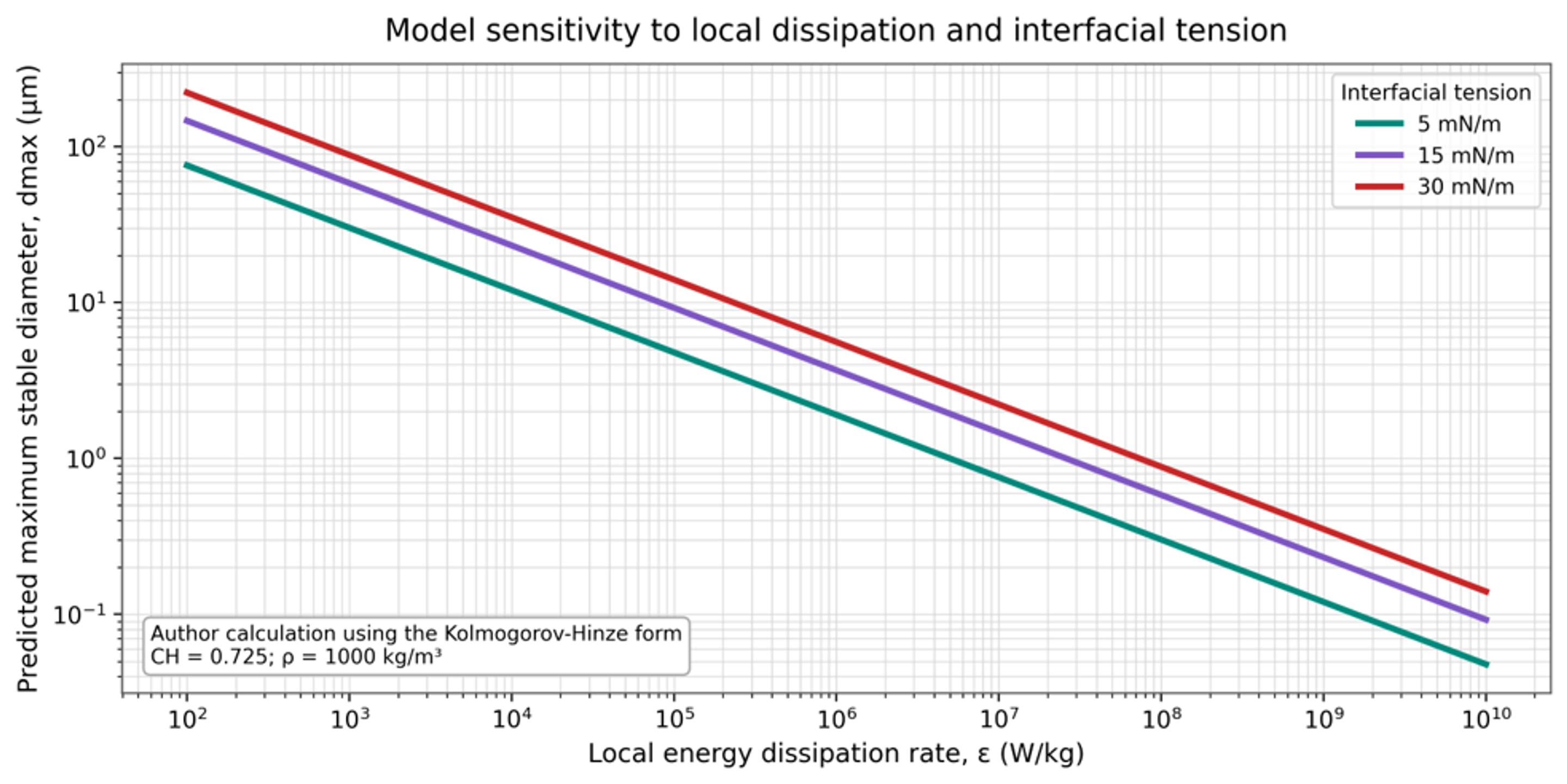
Figure 7. Model sensitivity of maximum stable droplet diameter to local energy dissipation and interfacial tension [9].