Fabrication of High Performance Catalysts by Controlled Flow Cavitation

2 Coupled Engineering and Materials Framework

Catalyst formation under cavitation is governed by two coupled histories. The hydrodynamic history includes acceleration through a restriction, low pressure exposure, bubble growth, turbulent shear, pressure recovery, collapse, and possible recycle. The material history includes supersaturation, nucleation, gel formation, fragmentation, solute transfer, crystallite growth, aggregation, washing, drying, and activation. A rigorous process description must document both histories.

The following equations provide an engineering framework for interpreting experiments, but they do not replace direct measurement. Loss coefficients, discharge coefficients, non-Newtonian rheology, dissolved gas, multiphase slip, and solids blockage can cause substantial deviations from ideal relations. Their principal value is to require explicit definition of pressure reference locations, geometry, fluid properties, and exposure time.

2.1 Pressure, Velocity, Reynolds Number, and Cavitation Number

For an incompressible liquid between an upstream point and a restriction throat, the mechanical energy balance can be written with a lumped irreversible loss term. Elevation is usually small in a compact processor, but it is retained in Equation 2.1 for completeness.

Here, $P_1$ and $P_t$ are the upstream and throat static pressures, $u_1$ and $u_t$ are the corresponding average velocities, $z$ is elevation, $\rho$ is liquid density, $g$ is gravitational acceleration, and $\mathrm{\Delta }{P}_L$ represents irreversible pressure loss. For a restriction with a calibrated discharge coefficient $C_d$, a useful estimate of throat velocity is given by Equation 2.2:

The Reynolds number describes the ratio of inertial to viscous effects and helps distinguish changes in jet structure and turbulence. For a noncircular throat, the hydraulic diameter $D_h$ should be reported.

Cavitation number is commonly used to compare the recovered pressure with vapor pressure relative to the throat dynamic pressure. The value is highly sensitive to the selected downstream pressure location. Investigators must state whether $P_r$ is measured immediately after the restriction, after pressure recovery, or in the recycle tank.

A low value of $\sigma$ generally favors vapor cavity formation, but it does not uniquely define collapse intensity. Increasing back pressure can shorten the bubble cloud and move collapse closer to the restriction. Increasing temperature raises vapor pressure and may increase cavity volume while simultaneously cushioning collapse with more vapor. Solids and dissolved gas can provide nuclei, attenuate pressure waves, or change the recovery profile. These competing effects explain why crystallite size and strain often respond nonmonotonically to an orifice setting.

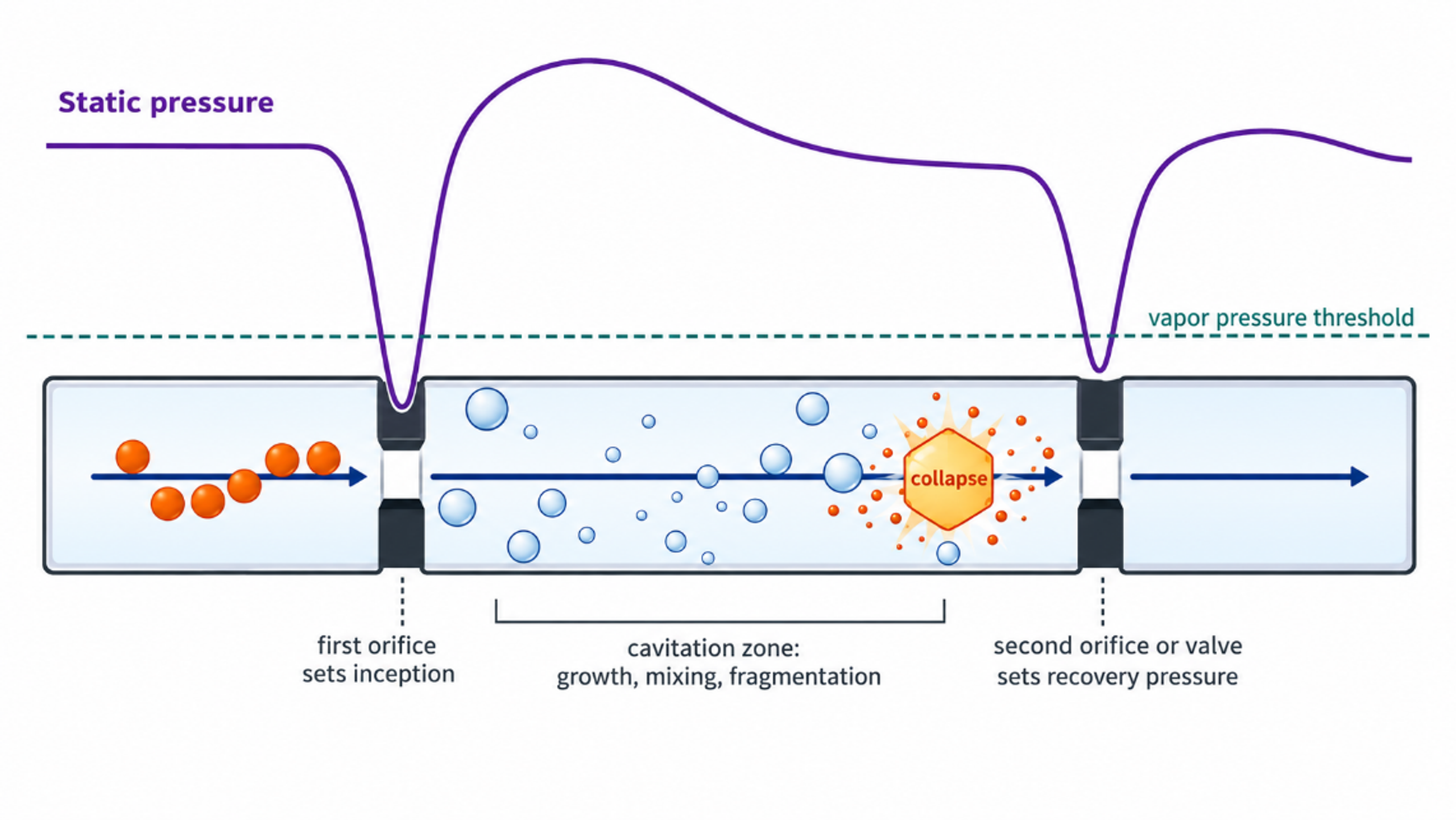
Figure 2.2. Conceptual pressure history and material events in a dual restriction cavitation processor. The pressure trace is schematic and is not a measured record. [29].

2.2 Bubble Growth, Collapse, and Particle Interaction

A spherical bubble in a Newtonian liquid can be described by the Rayleigh-Plesset equation:

Although a real CFC cloud contains interacting, nonspherical bubbles in a turbulent pressure field, the Rayleigh-Plesset relation identifies the principal roles of far field pressure, internal bubble pressure, surface tension, viscosity, and bubble radius [15-17,21].

For an ideal empty cavity that begins collapse at radius $R_{\max }$ under a constant pressure difference, the Rayleigh collapse time is approximated by Equation 2.6:

An order of magnitude estimate of mechanical work available from collapse is the pressure difference multiplied by the maximum cavity volume:

Only a fraction of this idealized work is transferred to a particle. Energy is partitioned among liquid compression, pressure waves, microjets, viscous dissipation, rebound, and thermal effects. Near a solid surface, asymmetric collapse can direct a microjet toward the particle or wall. In a slurry, particle-bubble contact depends on solids concentration, bubble population, particle size, surface wetting, and cloud residence time. Equation 2.7 should therefore be used for scaling and sensitivity analysis rather than to assign a unique particle temperature.

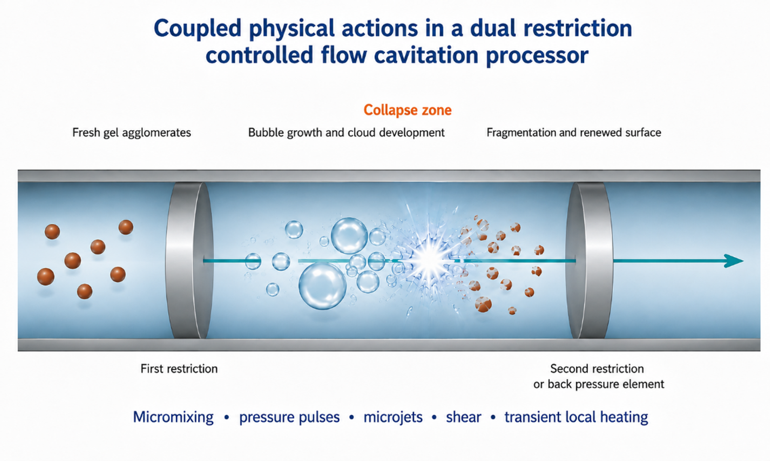
Figure 2.3. Coupled bubble and particle mechanisms in cavitation device. Rapid mixing, gel fragmentation, asymmetric collapse, surface renewal, and short local thermal events can act simultaneously. [29].

2.3 Hydraulic Power, Cumulative Exposure, and Residence Time

Hydraulic power transferred across the processor is estimated from pressure drop and volumetric flow. Pump efficiency must be included when electrical energy is compared:

For a recycle run, the specific hydraulic energy referred to isolated dry solids is given by Equation 2.9. The isolated mass rather than the theoretical precursor mass should be used so that yield loss is included:

The nominal number of loop passes, and the mean loop residence time are useful descriptors, provided that bypass volume and dead volume are included:

Single pass operation provides the clearest exposure definition and is preferred for kinetic studies. Recycle can increase cumulative treatment and narrow a weak agglomerate distribution, but it creates a distribution of exposure counts in which some particles pass through the restriction more often than others. Excessive recycle can promote dissolution and reprecipitation, pump heating, wear contamination, or irreversible agglomeration during warm storage. The optimum is therefore defined by a product quality window rather than by the maximum number of passes.

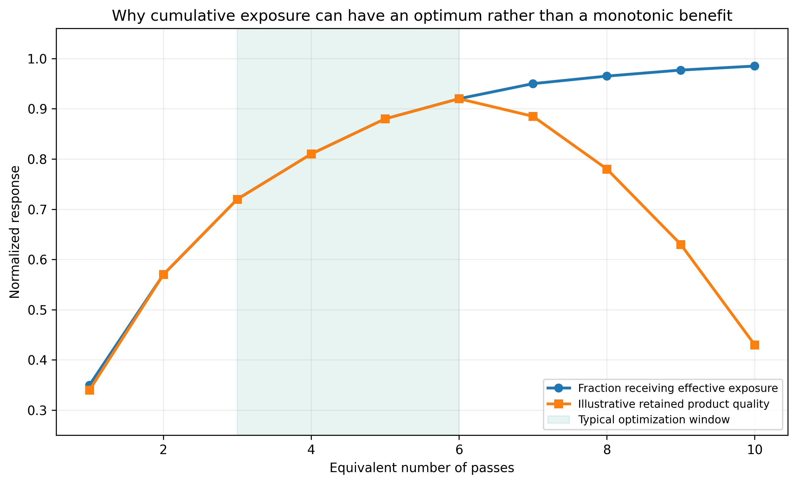
Figure 2.4. Conceptual relation between cumulative passes and product quality. Initial treatment improves mixing and deagglomeration, followed by a plateau and a possible overprocessing region. [29].

2.4 Micromixing, Supersaturation, Nucleation, and Growth

The smallest turbulent length scale is often estimated with the Kolmogorov relation. It is an ideal isotropic turbulence concept, but it provides a useful connection between local energy dissipation and the size of concentration fluctuations:

The associated mixing time scale is approximated by Equation 2.13:

Here, $\nu$ is kinematic viscosity and ${\epsilon }_h$ is the mass specific turbulent energy dissipation rate. The Microfluidics reaction study supplied with the source materials reported estimated mixing scales in the tens of nanometers and mixing times in the microsecond range for high pressure impinging jets [12]. Cavitation device geometries differ, but the study illustrates the degree to which intense, fixed geometry processing can reduce the lifetime of concentration gradients.

Supersaturation is the chemical driving force for precipitation. It may be represented as a concentration ratio or as relative excess concentration. The chosen definition must be stated:

Classical nucleation theory gives the critical radius of a spherical nucleus as Equation 2.15, where ${\gamma }_{sl}$ is the solid-liquid interfacial energy, $v_m$ is molar volume, $R_g$ is the gas constant, and $T$ is absolute temperature:

The nucleation rate is commonly represented in an Arrhenius form with a barrier $\mathrm{\Delta }{G}^{\ast }$:

Cavitation can modify both the preexponential factor and the effective nucleation barrier by changing local supersaturation, collision frequency, surface renewal, and heterogeneous nucleation sites. It can also accelerate growth by reducing diffusion resistance. These effects compete: higher nucleation density tends to reduce the mass available per nucleus, whereas enhanced transport and local warming can accelerate growth. Consequently, a smaller orifice, higher pressure, or lower cavitation number does not necessarily produce a smaller final crystallite.

Table 2.1. Engineering variables and the material forming responses they can influence

Engineering variable	Primary physical effect	Material response to measure	Common interpretation error
Upstream pressure	Changes jet velocity, pump heating, and pressure differential	Phase, agglomerate size, crystallite size, strain, yield	Assuming pressure alone equals cavitation intensity
Restriction geometry	Changes inception, jet contraction, cloud shape, and blockage sensitivity	Residence history, particle size distribution, erosion metals	Comparing only nominal diameter
Back pressure	Moves pressure recovery and collapse zone	Structure, temperature rise, erosion, repeatability	Assuming visible cavitation is the strongest collapse
Flow rate	Changes Reynolds number, renewal frequency, and pass time	Productivity, conversion, pass distribution	Ignoring loop inventory and bypass volume
Temperature	Changes viscosity, vapor pressure, kinetics, and ripening	Yield, phase, grain size, bulk temperature history	Treating temperature only as a fluid property
Solids loading	Changes attenuation, rheology, collision frequency, and pressure loss	Recovery, blockage, abrasion, agglomeration	Scaling dilute results directly to concentrated slurry
Feed timing	Sets the age of precipitate at first exposure	Composition uniformity, induction time, phase purity	Treating hydrodynamics separately from precipitation chemistry

2.5 Surface Area, Diffraction Size, Microstrain, and Active Area

For ideal, non-porous spherical particles of equivalent diameter $d$ and solid density ${\rho }_s$, the mass-specific surface area ($S_m$) is inversely proportional to the particle diameter:

This relation explains why small crystallites can expose a large fraction of surface atoms, but it does not predict BET area when pores, necks, platelets, support interfaces, or inaccessible internal surfaces are present. X-ray line broadening provides an independent estimate of crystallite size. The Scherrer equation is given in Equation 2.18:

If both finite size and strain contribute to broadening, the Williamson Hall form is useful:

Here, $K$ is the shape factor, $\lambda$ is X-ray wavelength, $\beta$ is corrected integral breadth, $\theta$ is the Bragg angle, and $ϵ$ is microstrain. Instrument broadening must be measured with a standard. Whole pattern refinement and microscopy are preferable to a single peak estimate. X-ray crystallite size, electron microscopy particle size, dynamic light scattering diameter, and laser diffraction agglomerate size describe different structural levels and should not be used interchangeably.

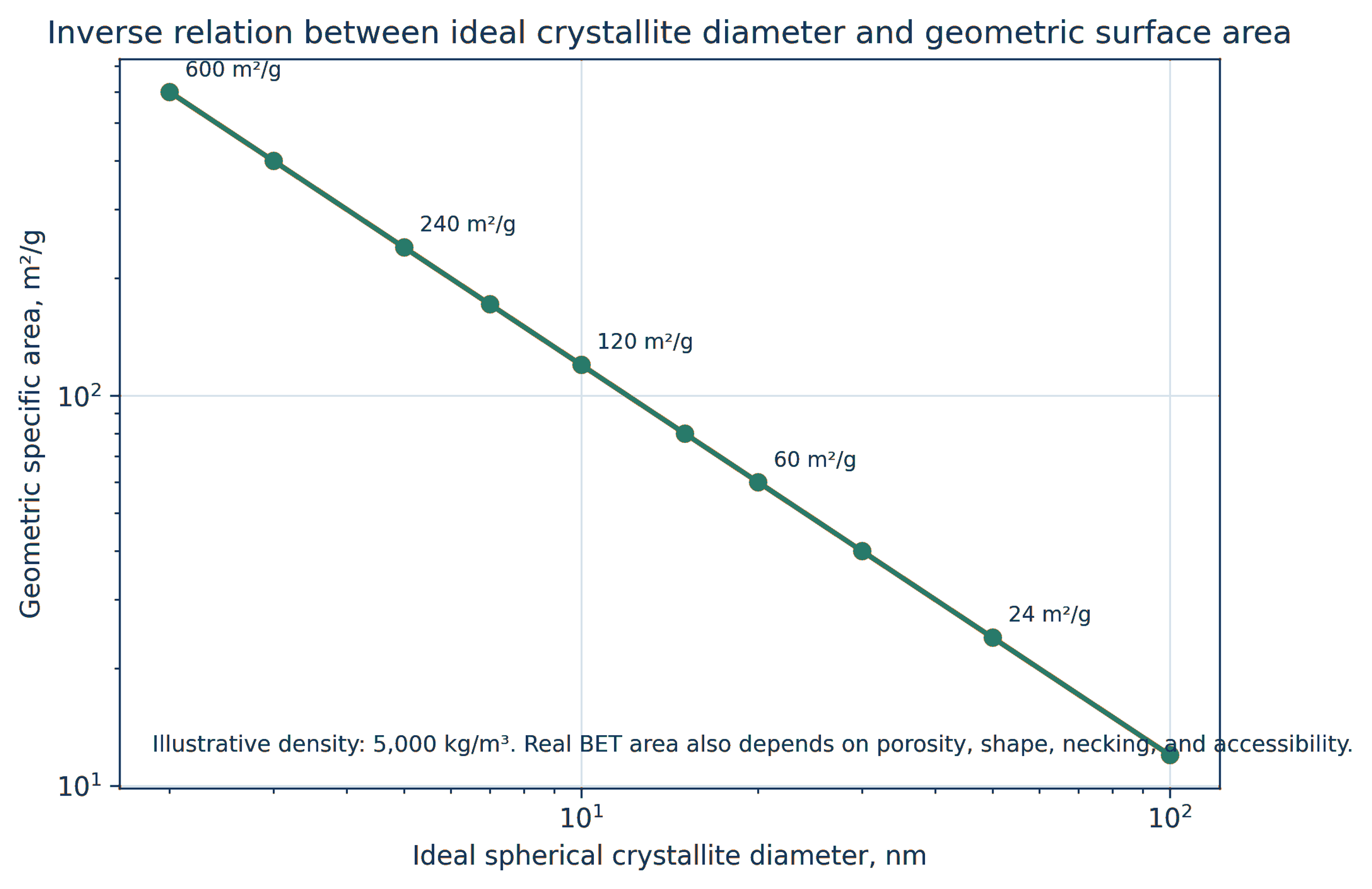
Figure 2.5. Ideal geometric area per unit mass as a function of crystallite diameter for representative oxide densities. The graph illustrates Equation 2.17. [29].

Table 2.2. Characterization methods and interpretation limits for CFC catalyst products

Method	Primary output	Required control	Important limitation
X ray diffraction	Phase, crystallite size, lattice parameter, microstrain	Instrument standard and multiple reflections	Insensitive to amorphous material and very small or dilute phases
Electron microscopy	Primary particles, agglomerates, interfaces, morphology	Representative fields and calibrated scale	Drying and sampling can bias morphology
BET gas adsorption	Accessible surface area and pore volume	Degassing protocol and adsorption model	Does not identify active chemical sites
Chemisorption	Metal dispersion and exposed active area	Defined reduction and adsorption stoichiometry	Strong support interaction can complicate uptake
X ray photoelectron spectroscopy	Surface composition and oxidation state	Charge correction and reference materials	Shallow sampling depth and air transfer effects
X ray absorption spectroscopy	Local coordination and oxidation state	Appropriate standards and in situ cell	Average signal can mask multiple populations
Particle size analysis	Hydrodynamic or optical agglomerate distribution	Refractive index, viscosity, dispersion protocol	Result depends strongly on dispersion state
ICP OES or ICP MS	Bulk composition and wear contamination	Digestion recovery and blanks	No information about spatial distribution