Engineering Calculations for Rotor-Stator Mixers

8 Pressure pulse energy and cavitation

8.1 Hydraulic specific work

For an incompressible liquid, a pressure difference $\mathrm{\Delta }{p}_p$ defines the hydraulic work scale per unit mass:

The resulting quantity has units of joules per kilogram and represents reversible pressure work for the stated pressure difference. Net energy transfer by an oscillating pressure field additionally depends on the displaced volume and its phase relative to pressure. A large pressure amplitude over a brief event can therefore correspond to little integrated work, while a smaller amplitude sustained over a larger displaced volume can transfer more energy. Hydraulic pressure work and stored wave energy require separate definitions.

Promtov developed calculation approaches for rotary impulse cavitation apparatus using specific measures of pressure pulses, pulsation, and cumulative action [8]. Application of these concepts requires explicit definitions of the integration interval, reference mass, and measured or modeled pressure and flow signals. A pressure amplitude has units of pressure and becomes an energy metric only through a stated physical conversion.

8.2 Acoustic energy and intensity

For a linear progressive plane wave in a uniform liquid, the cycle averaged total acoustic energy density, including kinetic and compressive contributions, is

Dividing that energy density by the liquid density gives the corresponding acoustic energy per unit mass:

Under the same progressive plane wave assumptions, the cycle averaged acoustic intensity is

Equations (8.2) to (8.4) use the root mean square pressure fluctuation. In a progressive plane wave, kinetic and compressive potential energy make equal contributions to the total energy density in Equation (8.2); compressive potential energy alone is half that total. The relations assume linear acoustics and the plane wave pressure to velocity relation. Close to a turbulent or cavitating workhead, reactive pressure fluctuations, standing waves, and multiphase effects can violate those conditions. The equations therefore provide reference wave measures, while local energy transfer requires the appropriate pressure and velocity field [16].

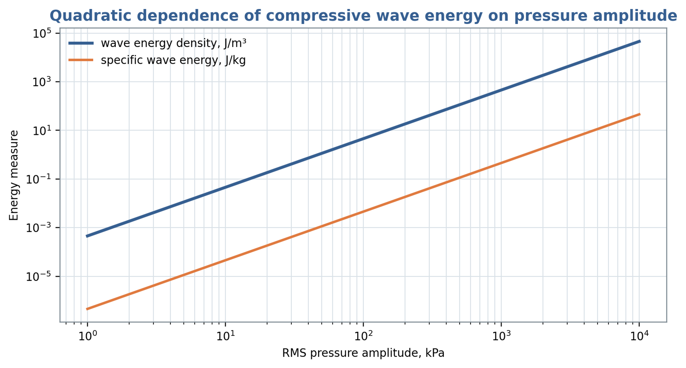
Figure 8.1. Total traveling wave energy per volume and per mass as functions of root mean square pressure amplitude, using Equations (8.2) and (8.3). The retained title refers to compressive energy; the plotted total includes equal kinetic and compressive contributions.

Table 8.1. Pressure related quantities that should not be confused

Quantity	Equation or definition	Units	Meaning
Pressure amplitude	$p_a$ or $p_{rms}^{\prime }$	Pa	Magnitude of fluctuation
Hydraulic specific work	$\mathrm{\Delta }p/\rho$	J/kg	Work associated with a pressure change
Total acoustic wave energy density	$p_{rms}^{\prime 2}/\left(\rho c^2\right)$	J/m³	Cycle averaged kinetic and compressive energy of a linear progressive plane wave
Acoustic intensity	$p_{rms}^{\prime 2}/(\rho c)$	W/m²	Cycle averaged energy flux of a linear progressive plane wave
Hydraulic power	$Q\mathrm{\Delta }p$	W	Product of mean flow and mean pressure difference; omits fluctuation covariance
Pulse fluence	$\int I_{a}dt$	J/m²	Time integrated wave energy per area

8.3 Cavitation number and minimum pressure

A commonly used cavitation number compares the available absolute pressure margin with a reference dynamic pressure:

Here, $p_{ref}$ is absolute pressure at a specified reference location, and $p_v$ is vapor pressure at the local liquid temperature. A smaller $\sigma$ indicates a smaller pressure margin relative to the chosen dynamic pressure. USACE guidance uses cavitation indices for hydraulic screening [17]. Rotating cavitation generators use related definitions, but inception depends on geometry, the velocity convention, nuclei, and the pressure history [18, 19]. A threshold measured for one apparatus should therefore be transferred only with evidence that these conditions are comparable.

A preliminary estimate of the minimum pressure can separate a mean local pressure depression from the negative part of a superimposed pulse:

Cavitation becomes possible as $p_{\text{min}}$ approaches vapor pressure, although nuclei and the duration of the pressure depression influence observable inception. In Equation (8.6), $C_p$ is defined as the positive magnitude of a geometry dependent pressure depression; its sign convention differs from the conventional signed local pressure coefficient. The quantity $p_a$ is the positive magnitude of the additional negative pulse. The steady and oscillatory contributions must be defined consistently to avoid counting the same pressure depression twice. A conservative estimate requires justified coefficients and a credible coincidence of their adverse contributions.

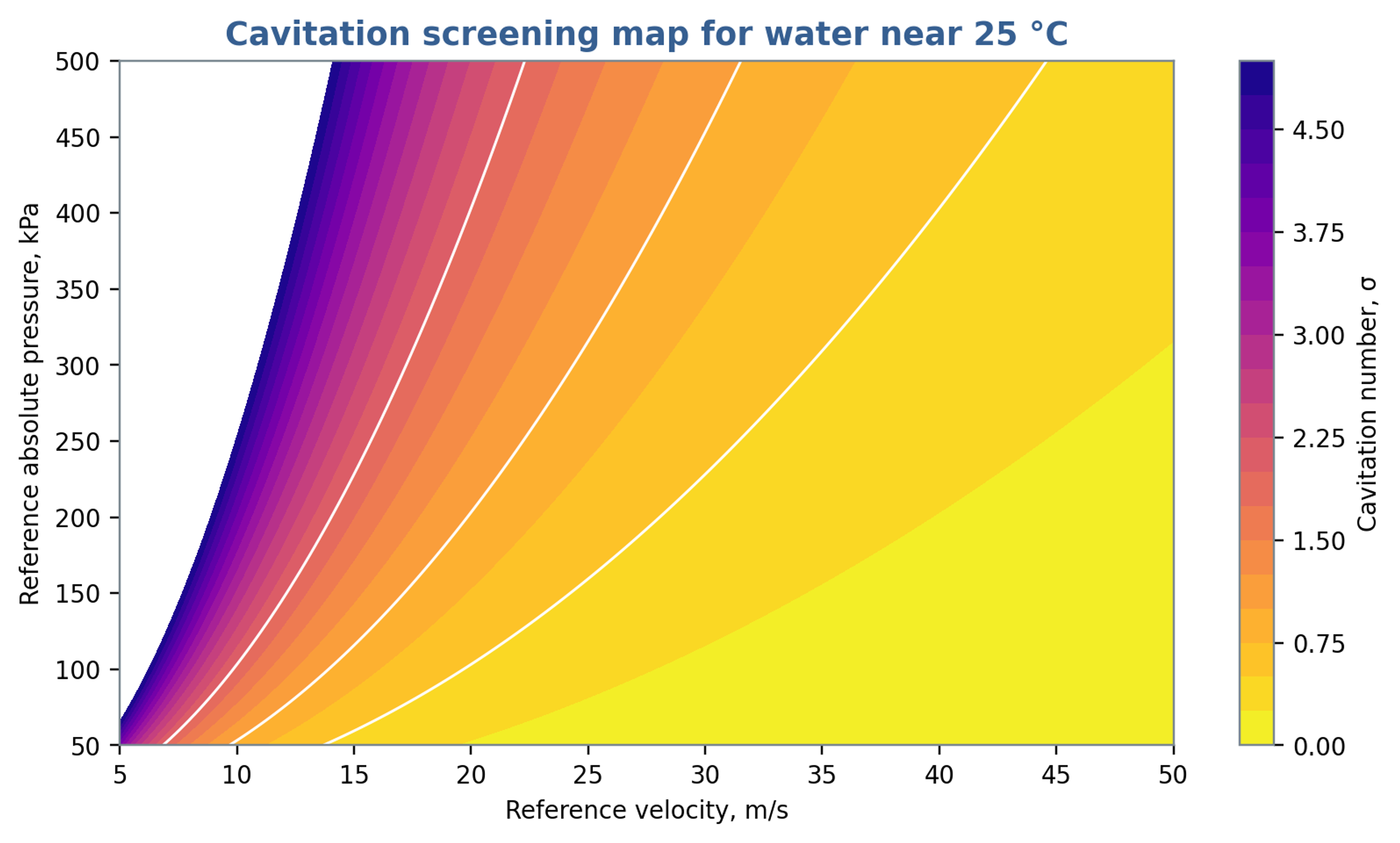
Figure 8.2. Cavitation number calculated from Equation (8.5) using a vapor pressure of 3.2 kPa, representative of water near 25 °C. Pressure is absolute. The contours do not define a universal cavitation inception threshold.

8.4 Bubble dynamics and collapse scales

For an isolated spherical bubble in an effectively infinite incompressible Newtonian liquid, with uniform internal pressure, the Rayleigh Plesset equation describes radial motion:

The symbols $R$, $p_B$, $p_{\infty }$, and $\gamma$ denote bubble radius, internal bubble pressure, imposed far field liquid pressure, and surface tension, respectively [19, 20, 21]. A calculation requires the complete external pressure history, initial radius and wall velocity, and a closure for the gas and vapor pressure inside the bubble. Gas content, thermal response, viscosity, and surface tension influence growth and collapse. Liquid compressibility, strong deformation, and nearby boundaries require more detailed models when their effects are appreciable [19].

For a spherical vapor cavity collapsing from rest under a constant positive pressure difference $p_{\infty }-p_v$, with gas cushioning, viscosity, surface tension, and liquid compressibility neglected, the ideal Rayleigh collapse time is

The product of the maximum cavity volume and its collapse driving pressure gives a characteristic pressure work scale:

Equation (8.9) estimates a cavity energy scale rather than a universal bound on useful treatment energy. Its conversion into sound, rebound, liquid motion, heat, deformation, and viscous dissipation depends on the collapse conditions. Nearby solid surfaces promote asymmetric collapse and can direct a liquid microjet toward the material, producing erosion [19]. Dense clouds introduce interactions and shielding that cannot be represented by a set of independent spherical bubbles without additional coupling. These limitations should accompany any conversion from bubble size to process performance.

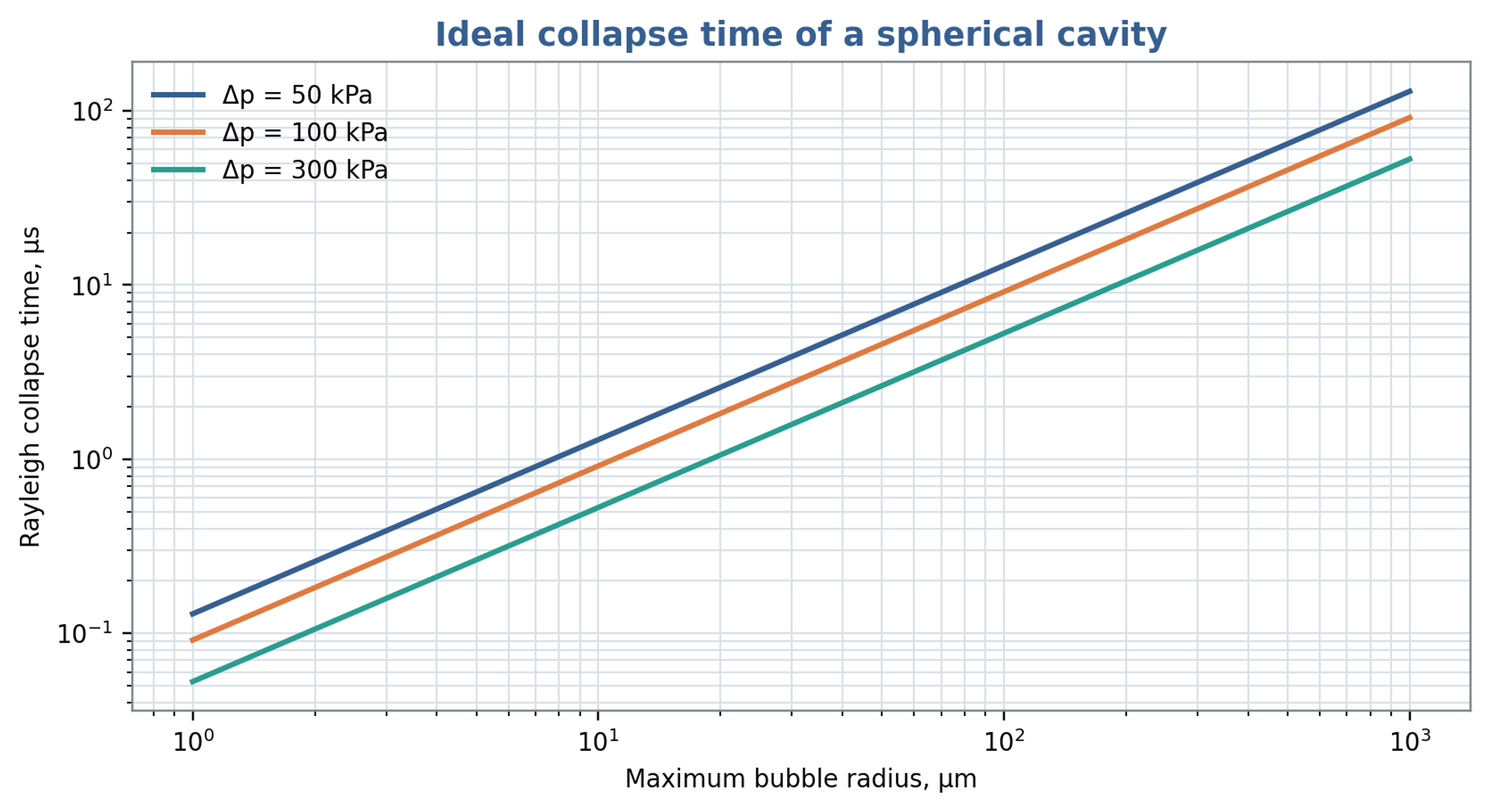
Figure 8.3. Ideal Rayleigh collapse time versus maximum cavity radius and imposed pressure difference, calculated from Equation (8.8). The model neglects gas cushioning, viscosity, surface tension and liquid compressibility.

8.5 Cumulative exposure and process response

A useful cumulative exposure metric should retain pressure amplitude, event duration, event count, and the processed mass. Possible empirical measures include time integrated exposure below a declared pressure threshold or a calibrated acoustic measure within a selected frequency band, referenced to a comparable noncavitating baseline. Product response can then be assessed against exposure, specific shaft energy, and pass count. These metrics require experimental calibration because pressure fluctuations and acoustic emissions do not uniquely determine chemical, biological, or particle response. Nuclei, gas content, reaction kinetics, and device geometry remain relevant explanatory variables.

Promtov and Akulin associated heat generation in a rotor impulse apparatus with cavitation and pressure pulse processes [22]. Assessment of that interpretation requires a complete energy balance. In a closed system, mechanical energy dissipated through shear, turbulence, restriction losses, or bubble motion ultimately contributes to heating, subject to heat removal and energy exported from the boundary. A measured temperature rise therefore quantifies retained thermal energy but does not, by itself, establish which intermediate mechanism dominated.

8.6 Relation to droplet breakup

A product response should accompany hydraulic and power calculations when the objective is emulsification. Hall et al. investigated silicone oil emulsions over a broad range of dispersed phase viscosities in an inline mixer. Rotor speed and dispersed phase viscosity strongly influenced mean droplet size, whereas flow rate had a weaker effect within the tested range. Their interpretation distinguished droplets mainly affected by turbulent inertial stresses from smaller droplets for which viscous effects also became relevant. These observations support specifying formulation properties and the required droplet size distribution alongside nominal gap shear and specific energy. The published trends apply to the investigated formulations and operating conditions and do not define a universal throughput optimum [23].

The location and duration of intense stress influence the interpretation of nominal residence time. Håkansson et al. compared turbulent stress estimates derived from particle image velocimetry with visual observations of droplet breakup. They identified intense regions associated with flow entering a stator hole, the shear layers of the exiting jet and a larger structure produced after rotor blockage. The predicted region near the hole exit agreed with observed breakup locations, although mean stress estimates did not explain every event. This evidence supports interpreting the mixer as a spatially and temporally varying stress field. A nominal pulse count or average residence time should therefore be reported as an exposure descriptor rather than a direct measure of successful fragmentation [24].