Engineering Calculations for Rotor-Stator Mixers

Geometry and unsteady flow in relation to pressure pulsation, cavitation and power consumption

O. Kozyuk, Ph.D

Abstract

Rotor-stator mixers convert shaft work into circulation, deformation, turbulent motion, pressure fluctuations and heat. Their engineering description therefore requires a consistent connection between working geometry, rotational speed, flow rate, fluid properties and the pressure boundary conditions. This article develops a calculation framework that combines feature passage kinematics, time dependent overlap area, a lumped model of passage flow, cylindrical Couette flow, dimensionless operating parameters, cavitation screening and an overall energy balance. Hydraulic pressure work is distinguished from the energy of a traveling acoustic wave, and the limits of simplified bubble and gap models are stated explicitly.

The framework is supplemented by published experimental and computational studies of power consumption, flow distribution, emulsification and scale up. A screening example for an 80 mm rotor operating at 6000 rpm gives a tip speed of 25.13 m/s, a local feature passage frequency of 800 Hz, a nominal gap shear rate of 5.03 × 10⁴ s⁻¹ and a cavitation number of approximately 0.62 under the specified reference conditions. These results establish kinematic and hydraulic scales; they do not independently establish cavitation inception, shaft power or product performance. The analysis shows that reliable design depends on geometry specific validation and on a power balance with consistent boundaries, complemented by measurements of pressure, temperature and the product response.

Keywords: rotor-stator mixer; unsteady flow; pressure pulsation; cavitation; shaft power; engineering calculation; scale up.

1 Introduction

Rotor-stator mixers impose rapid deformation while transporting liquid through a closely spaced moving and stationary assembly. Even at constant mean throughput, the local flow near a slot or tooth contains a periodically forced component. Passage opening and closure generate velocity and pressure fluctuations at feature passage frequencies and their harmonics. The resulting pressure history also depends on liquid inertia, hydraulic resistance, gas content, compressibility, housing compliance and the connected piping [1, 2, 3]. These coupled effects explain why nominal speed alone is insufficient to characterize the process.

The terminology reflects different emphases within this class of equipment. Russian and Ukrainian publications commonly describe rotary pulse, rotor pulse and flow modulation apparatus, whereas English language literature often uses rotor-stator mixer, high shear mixer or inline homogenizer. Transfer of a calculation method requires correspondence between the physical flow paths. Cylindrical slotted members, intermeshing rows of teeth, perforated screens and devices with axial working clearances have different pumping, leakage and dissipation mechanisms. The active passages, minimum simultaneous opening area, wetted surfaces and pressure recovery regions must therefore be specified for each configuration.

Patent SU829155A1 describes concentric slotted rotating and stationary cylinders and identifies flow pulsation, turbulence, shear and cavitation as possible effects of passage through the moving openings [4]. Patent US5632596A describes another arrangement with concentric rows of shallow teeth and radial grooves [5]. These examples establish geometric distinctions relevant to calculation; a patent description by itself does not validate a performance correlation. Tooth count, opening width, active height, clearance and row arrangement must be specified independently of the rotor diameter.

The objective of this article is to connect the geometry of periodic mixing heads with a hierarchy of kinematic, hydraulic and energy calculations. The analysis proceeds from quantities that follow directly from the design dimensions to quantities that require empirical closure. The distinction is useful when evaluating a proposed mixer because a calculated event frequency, shear scale or pressure margin provides a testable prediction, while the power demand and final product properties additionally depend on the realized flow and material response.

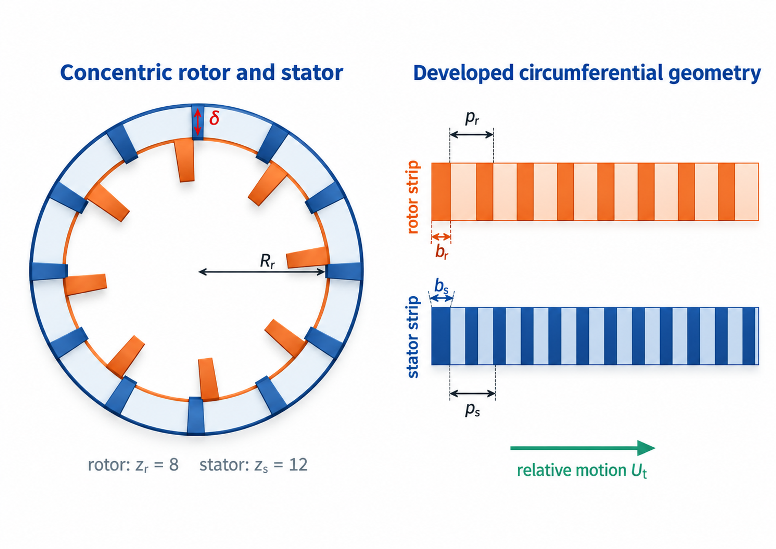
Figure 1.1. Representative cylindrical calculation geometry and developed circumferential patterns. The schematic identifies rotor and stator features, clearance, pitch, opening width and relative motion.

Table 1.1. Minimum input data for an engineering calculation

Data group	Required quantities	Why they are needed
Rotor geometry	Outside diameter, active radius, axial height, number of teeth or slots, slot width and depth, number of rows	Determines tip speed, opening area, event frequency, wetted area, and rotational drag
Stator geometry	Inside diameter, opening count, opening width and height, open area, edge thickness	Determines restriction, jet velocity, pressure loss, and overlap with the rotor pattern
Clearances	Radial gap, axial gap, runout allowance, thermal growth allowance	Controls nominal shear, leakage, friction, contact risk, and local pressure
Operating point	Rotor speed, flow rate, inlet and outlet absolute pressure, temperature	Defines kinematics, residence time, hydraulic power, cavitation margin, and heat balance
Fluid properties	Density, dynamic viscosity, kinematic viscosity, vapor pressure, speed of sound, heat capacity, surface tension	Required for Reynolds, Womersley, cavitation, bubble, acoustic, and thermal calculations
Measured performance	Torque or electrical input, no load power, pressure waveform, flow waveform, vibration and sound	Separates mechanical losses from fluid power and validates the unsteady model

SI units are used throughout. Rotational frequency $N$ is expressed in revolutions per second, whereas shaft speed $n$ is expressed in revolutions per minute. The conversion is

The corresponding angular speed is

For active diameter $D$ and radius $R=D/2$, the peripheral velocity is

Tip speed establishes a useful kinematic scale. Its interpretation requires the gap width, opening area, flow rate, pressure and exposure time because those quantities determine how the available motion is transferred to the liquid.

2 Calculation framework and model boundaries

The calculation proceeds from geometry and kinematics to hydraulics, energy conversion, operating limits and validation. Geometric analysis determines the active radii, pitch, clearances and time dependent openings. Hydraulic analysis then estimates the mean flow and the fluctuations within passages and gaps. Torque, pressure and flow define the power balance, from which specific energy and heating can be evaluated. The final stage compares these predictions with measured pressure, shaft load, temperature and product properties.

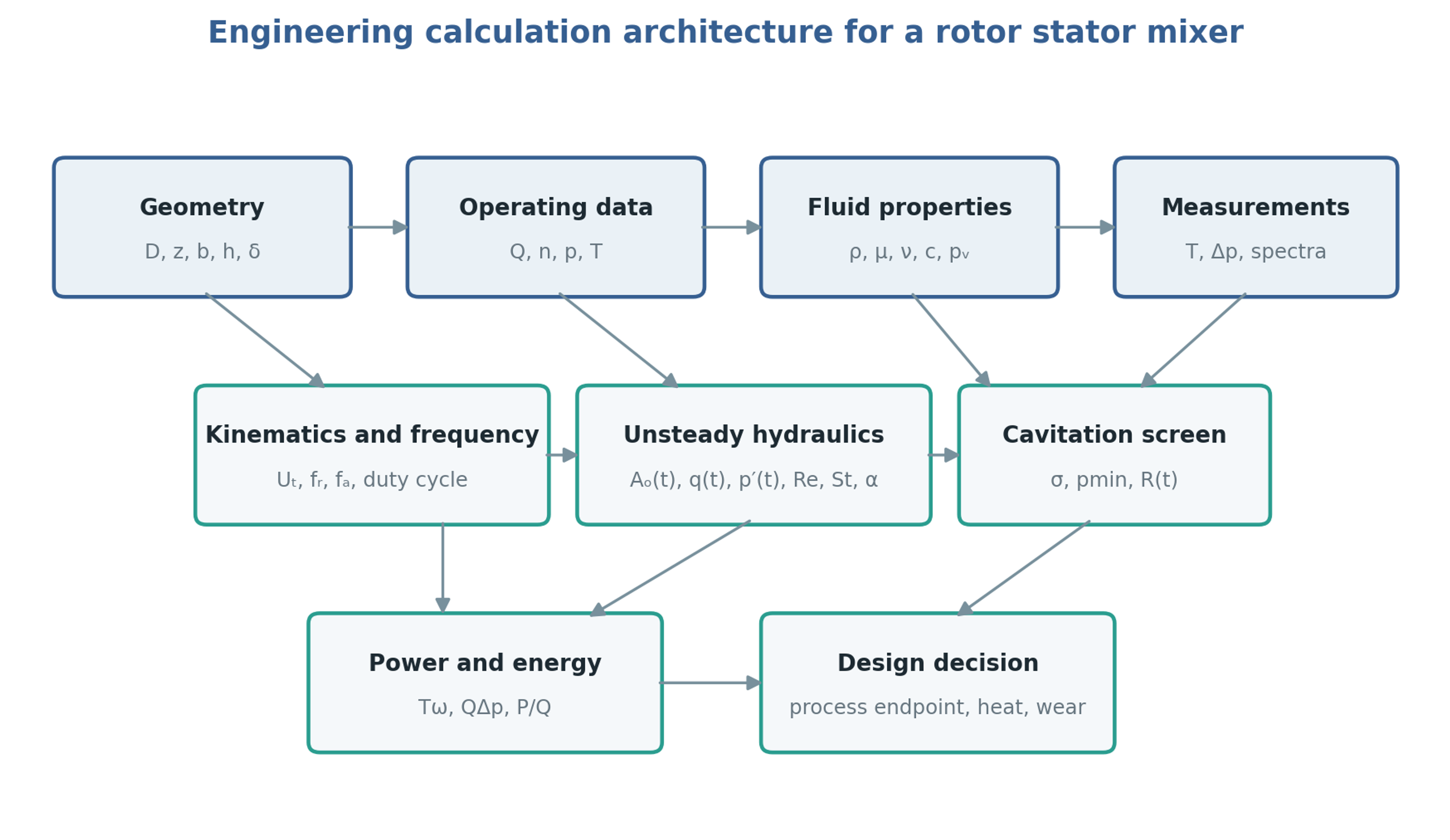
Figure 2.1. Calculation structure linking geometry, operating conditions, fluid properties and measurements to hydraulic and energy analysis. Diagram synthesized from the methods in [1, 7, 8, 9, 10].

The control volume determines the meaning of each calculated power or pressure difference. In batch operation it may enclose the working head or the entire vessel. In an inline system it may enclose the mixer housing or a larger recirculation circuit containing valves, pipework and a heat exchanger. A pressure fluctuation measured close to the stator can be attenuated before reaching a remote gauge, while a piping resonance can amplify a selected harmonic. The volume, compliance and hydraulic resistance of the external circuit should therefore be included when they influence the transient response.

The preliminary models use the following assumptions, which must be matched to the selected operating regime.

Mean flow and viscous shear are evaluated for a Newtonian liquid with negligible density variation.

Weak compressibility is retained when estimating pressure waves and rapid hydraulic transients.

The nominal rotor and stator surfaces are concentric, with a uniform working clearance.

A sharp edged orifice approximation is used for openings unless a measured discharge coefficient is available.

Fluid properties are evaluated at a stated process temperature and composition.

Cavitation screening uses absolute pressure and is checked against measurements or a validated transient model.

Power and flow correlations are applied within their demonstrated geometric and hydrodynamic ranges.

Constitutive and flow models require additional treatment for non Newtonian or viscoelastic products, substantial gas fractions, concentrated slurries, flexible components and developed cavitation. In these cases the same calculation structure remains useful, but its coefficients and closure relations require representative experiments or resolved numerical analysis. Mechanical integrity and product performance must be assessed alongside the hydraulic predictions.

Table 2.1. Calculation levels and appropriate uses

Level	Method	Appropriate use	Main limitation
Screening	Tip speed, nominal shear, open area, cavitation number, $P/Q$	Early selection and test matrix design	Does not resolve local flow or pressure
One dimensional transient	Hydraulic inertance, resistance, time varying opening, pressure source	Pulse amplitude, phase, and system interaction	Requires calibrated loss and compliance terms
Three dimensional transient or periodic CFD	Sliding mesh or resolved rotor position	Local jets, wakes, pressure minima, torque	Computational cost and turbulence or cavitation model uncertainty
Full experimental characterization	Synchronized torque, pressure, flow, temperature, spectra, product response	Design validation and scale up	Apparatus and fluid specific

2.1 Extension to fluids with yield stress

The constant viscosity approximation requires reconsideration when the processed material exhibits yield stress or strong shear dependence. Ayas et al. combined experiments with laminar computational modeling for a collagen solution represented by a Herschel and Bulkley constitutive relation in a particular inline mixer. They determined power and characteristic shear coefficients and examined how axial clearance affected the shear distribution. A clearance change could modify the local shear characterization while producing little change in total power over the investigated range. Their results show why integral power alone is insufficient to describe treatment uniformity in such fluids. The fitted coefficients and small hydraulic power contribution remain specific to the tested material and mixer geometry [11].

3 Working geometry

3.1 Feature count and circumferential pitch

For a cylindrical rotor of outside diameter $D_r$ with $z_r$ equally spaced features, the circumferential pitch is

If the circumferential clear opening is $b_r$, the tooth or bridge width is

Equivalent definitions apply to the stationary member. Rectangular stator slots of width $b_s$ and active height $h_s$ have the total geometric area

For an ideal uniform pattern, the circumferential open fraction is

Equation (3.4) defines geometry. Hydraulic contraction, wall thickness, upstream swirl, blockage, gas cavities and uneven flow distribution affect the effective discharge area. The product $C_d{A}_s$ is commonly used in an orifice representation, with $C_d$ determined from an applicable correlation or a calibration. The coefficient must not be interpreted as a change in the manufactured opening dimensions.

At fixed diameter, a larger feature count reduces the circumferential pitch. If opening width is held constant, the open fraction increases and the intervening bridges become narrower. If open fraction is held constant, both opening and bridge widths decrease. The accompanying increase in passage frequency must be considered together with drag, clogging, manufacturing tolerances and wear. The examples in US5632596A include 45 radial grooves at 8 degree intervals and demonstrate that tooth height and the number of concentric rows can vary independently of outside diameter [5].

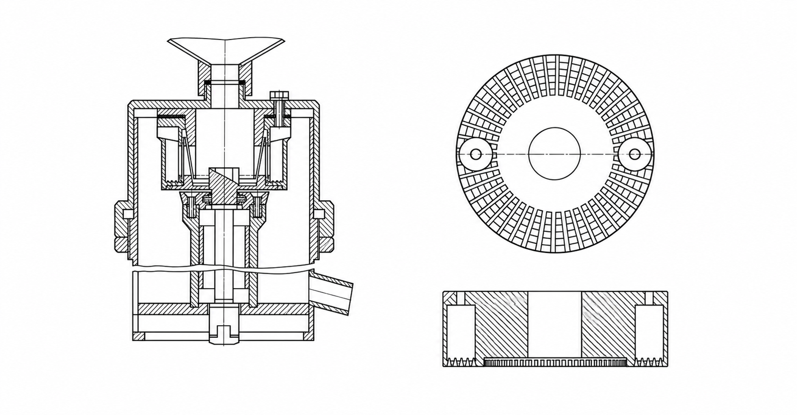
Figure 3.1. Rotor-stator architectures shown as simplified technical illustrations. Left, the apparatus disclosed in SU829155A1. Right, plan and sectional views of the low profile toothed stator disclosed in US5632596A.

Table 3.1. Geometric variables and their first order effects

Variable	Increase generally causes	Countervailing effect or risk
Rotor diameter	Higher tip speed at fixed rpm, larger wetted area, greater pumping potential	Strong increase in torque and power; larger shaft and bearings
Rotor feature count	Higher local passage frequency and edge density	Smaller bridges, clogging, manufacturing tolerance sensitivity
Stator opening count	More distributed jets and larger potential area	Reduced individual jet momentum if total flow is fixed
Slot width	Larger open area and longer opening duration	Lower local velocity and weaker pressure modulation at the same flow
Slot depth or active height	Larger flow area and wetted surface	Higher drag and larger trapped volume
Radial gap	Lower nominal shear and contact risk	More leakage, reduced pressure modulation, weaker local stress
Number of rows	More repeated energy input events	Greater pressure loss, heat, residence time, and cleaning difficulty

3.2 Radial clearance and manufacturing allowance

For rotor radius $R_r$ and stator radius $R_s$, the nominal radial clearance is

The dimensionless clearance may be expressed as $\delta /R_r$ or $2\delta /D_r$. The nominal drawing value differs from the smallest clearance reached during operation. Shaft runout, bearing play, housing deflection, thermal expansion, eccentric assembly and entrained particles can reduce the local gap. A tolerance assessment should consequently include both assembly conditions and the expected temperature distribution during operation.

Reducing the gap increases the nominal velocity gradient and viscous stress while restricting leakage between adjacent passages. It can strengthen area modulation, but it can also increase drag, heating, erosion and the probability of contact. Chervyakov and Yudaev explicitly account for flow through finite clearances while the main stator channel is covered [1]. This treatment is relevant because complete hydraulic closure is generally inconsistent with nonzero radial or axial leakage paths.

Clearance selection should begin with the manufacturing and mechanical limits and then be evaluated hydraulically. The selected gap must remain achievable under the combined effects of speed, load, temperature and wear. Predictions based on a clearance smaller than the maintained operating gap will overstate nominal shear and the degree of passage closure.

3.3 Time dependent overlap area

A compact representation of the periodic effective opening is

where ${\overline{A}}_o$ denotes the mean opening, $m_A$ is an area modulation index, $g$ is a periodic function of zero mean and unit characteristic amplitude, $f_A$ is the selected overlap frequency, and ${\phi }_A$ is the phase. A sinusoidal function supports linear analysis, whereas triangular or trapezoidal functions can better approximate rectangular openings. Piecewise area models can account for progressive exposure and finite leakage [1]. The selected representation must reproduce the minimum, maximum and mean areas, together with the opening duration; it must also remain nonnegative throughout the cycle.

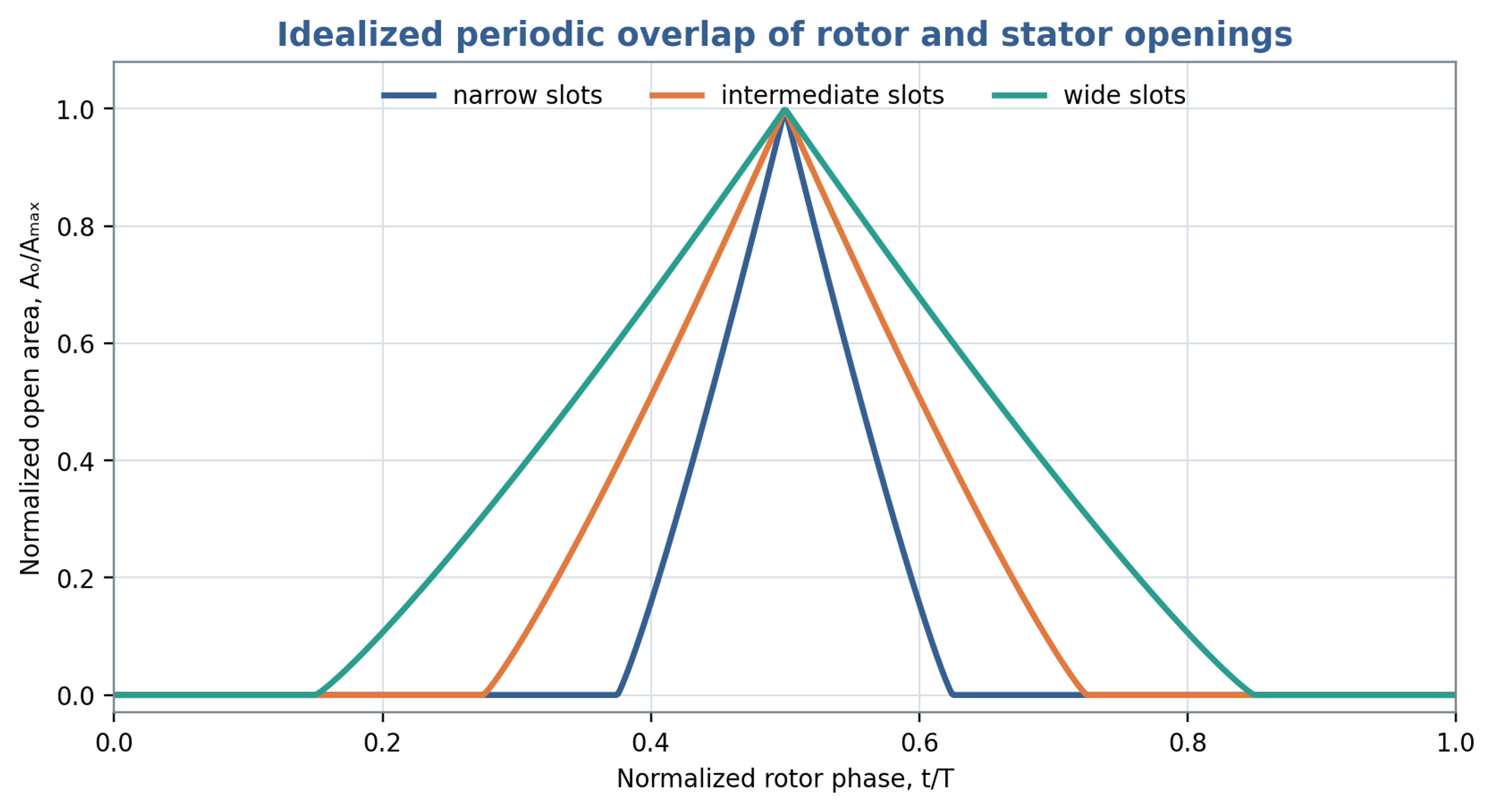
Figure 3.2. Normalized overlap area for narrow, intermediate and wide opening windows. These idealized curves illustrate geometric modulation rather than measured apparatus performance.

The area waveform influences both jet acceleration and the harmonic content of the forcing. Narrow exposure windows concentrate the opening event into a shorter part of the cycle. Wider windows extend the period of flow and generally reduce the relative importance of rapid opening and closure. Figure 3.2 illustrates these geometric effects. The preferred configuration depends on the required throughput, pressure modulation, thermal limit and resistance to blockage.

3.4 Evidence from systematic geometry changes

Stator geometry should be assessed through controlled changes in both the perforations and the inlet boundary. John et al. used computational models, supported by measured power, to relate workhead dimensions to flow and power characteristics. Within the limited hole sizes investigated at constant total opening area, the hole hydraulic radius did not independently change one fitted power and flow coefficient. This result does not make hole size irrelevant for arbitrary screens. The authors identified stronger fluctuations as a reason to use transient calculations or several rotor positions when extending the hole size range. The engineering implication is to document total opening area, individual passage dimensions and inlet configuration together when comparing heads [12].

4 Flow pulsation frequencies

4.1 Local feature passage

At a stationary observation point, passage of $z_r$ identical rotor features produces the kinematic frequency

This frequency commonly appears in a pressure signal measured near one stator opening. Its amplitude depends on the rotor and stator patterns and on the hydraulic response. Harmonics at $2f_r$, $3f_r$ and higher multiples arise from departures of the local waveform from a sinusoid. A kinematic event frequency therefore specifies a candidate spectral component, while its measured amplitude requires a flow model or an experiment.

4.2 Integrated overlap and exposure time

The summed overlap around the circumference has additional symmetry. For ideal uniformly spaced rotor and stator patterns with feature counts $z_r$ and $z_s$, a repeat frequency associated with their common rotational symmetry is

Equation (4.2) gives a symmetry repeat frequency of the integrated opening pattern. It does not guarantee a nonzero fundamental in the measured pressure or even a varying total open area. Particular opening widths can cancel the corresponding Fourier coefficient, and the first surviving component can occur at a higher harmonic. Asymmetry, maldistribution, sensor position, staggered rows and hydraulic coupling can instead emphasize $f_r$, $f_s$, shaft frequency or other combinations. The reported frequency must identify whether it refers to a local passage event, a geometric repeat or an observed pressure component.

For characteristic effective width $b_e$ and relative tangential velocity $U_t$, a nominal exposure time is

The width $b_e$ depends on both opening widths and on whether exposure means any overlap or a selected effective area. The duty ratio $t_o{f}_A$ is meaningful only when $f_A$ refers to successive equivalent events of that same opening definition. Local exposure time should not be combined automatically with a frequency calculated from the summed circumferential area.

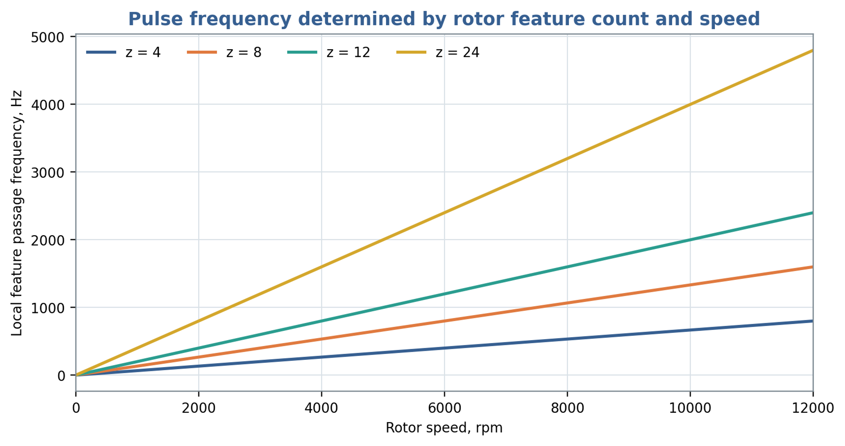
Figure 4.1. Local rotor feature passage frequency as a function of shaft speed and feature count, calculated from Equation (4.1).

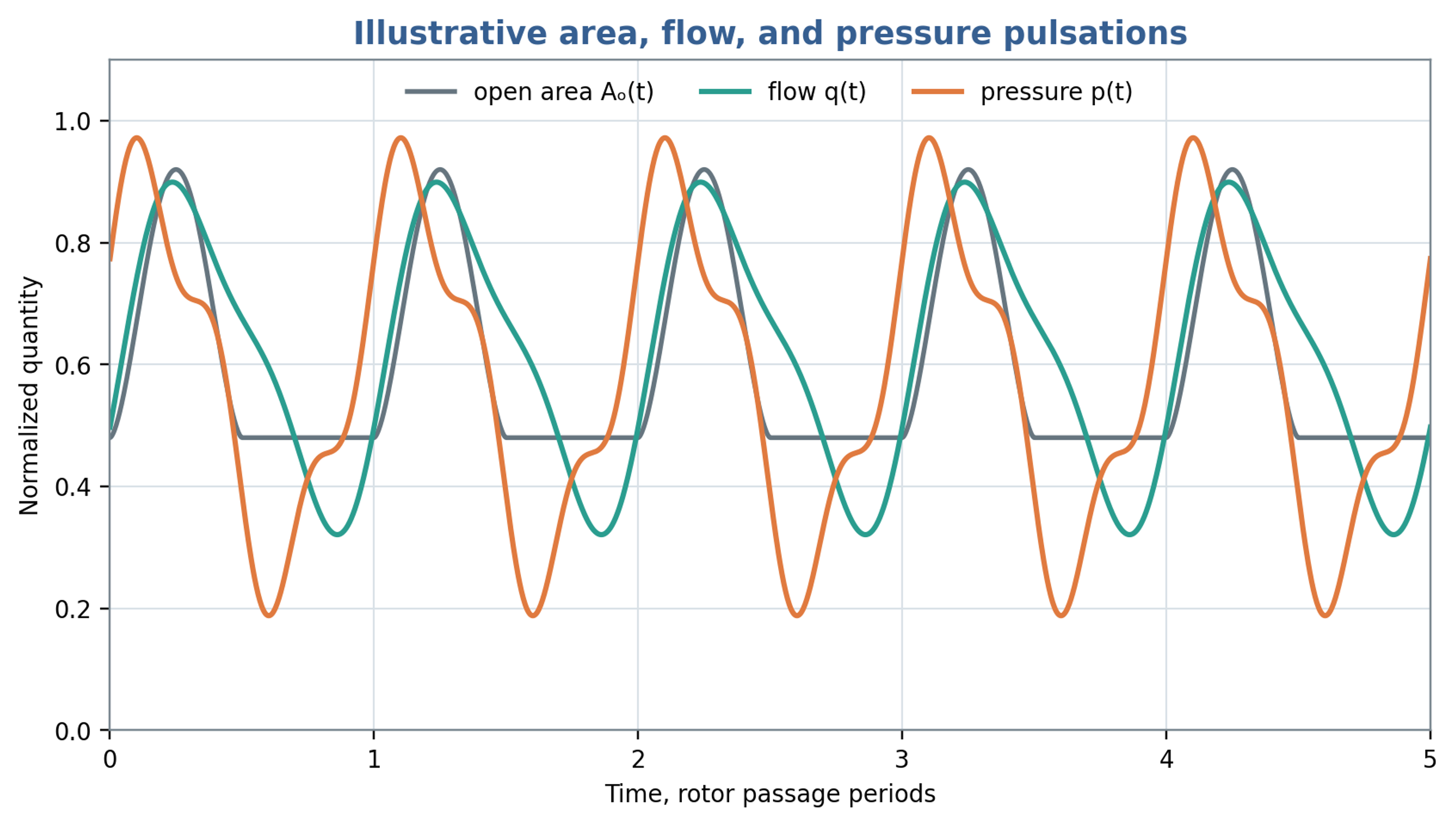
Figure 4.2. Illustrative normalized opening area, flow and pressure waveforms. Hydraulic inertia and resistance introduce phase differences between the signals. The traces are model examples.

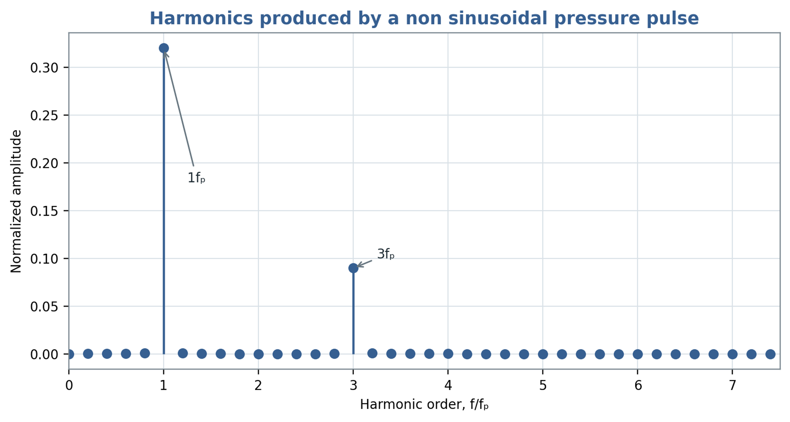
Figure 4.3. Harmonic spectrum of the illustrative pressure waveform. Spectral amplitudes refer to the specified example and are not a universal mixer spectrum.

Table 4.1. Frequency definitions used in rotor stator calculations

Frequency	Definition	Typical use
Shaft frequency	$N=n/60$	Mechanical vibration, imbalance, once per revolution asymmetry
Rotor local passage	$z_{r}N$	Pressure or velocity near a fixed stator location
Stator interaction count	$z_{s}N$ when viewed from a rotor attached sensor or repeated rotor path	Relative pattern interaction
Integrated overlap symmetry repeat	$\text{lcm}(z_r,z_s)N$ for ideal uniform patterns	Symmetry of total opening area; verify nonzero harmonics
Harmonics	$k{f}_p$, $k=\mathrm{2,3},\dots$	Sharp opening and closing, resonance, noise
Structural natural frequency	Determined from housing, shaft, pipe, and supports	Resonance screening

5 Unsteady flow in working passages

5.1 Conservation equations

Mass conservation provides the starting point for the unsteady flow model. Retaining density variation gives the continuity equation for a weakly compressible liquid:

For a Newtonian liquid of spatially uniform viscosity, with dilatational viscous stresses neglected at leading order, the momentum equation in an inertial reference frame is

Transformation to a reference frame rotating with the rotor introduces centrifugal and Coriolis accelerations. Chervyakov and Yudaev formulate the problem using the cylindrical Navier Stokes equations and then develop approximations for flow in rotating rectangular channels [1]. If circumferential relative motion and transverse variations are neglected, the radial component can be represented by

The centrifugal term ${\omega }^{2}r$ contributes to outward acceleration, whereas the pressure gradient responds to the imposed boundary pressures and the changing hydraulic restriction. Equation (5.3) retains only radial viscous derivatives. It therefore does not resolve the wall friction associated with velocity gradients across the width and height of an actual channel. Those effects require a resolved cross section or a separate resistance closure. Periodic variation of the downstream opening repeatedly accelerates and decelerates the liquid even when shaft speed is constant.

5.2 Hydraulic inertance and resistance

For preliminary calculations, the distributed channel problem can be reduced to a hydraulic element containing inertance, linear viscous resistance, and a nonlinear local loss. The governing balance for one modeled passage is

where $q$ is the instantaneous volumetric flow, $I_h$ is hydraulic inertance, $R_h$ is linear hydraulic resistance, $K$ is a local loss coefficient, $A$ is the reference flow area, and $\mathrm{\Delta }{p}_d(t)$ is the net driving pressure, including the centrifugal contribution and imposed system pressures. The signed nonlinear term opposes either direction of flow. For a liquid column of effective length $l_e$ and fixed reference area $A$, the inertance is

For fully developed laminar flow between parallel stationary surfaces separated by a small gap $h$, with channel width satisfying $w\gg h$, the linear hydraulic resistance is approximately

The nonlinear term generally becomes important for short restrictions and rapidly moving jets. The coefficient $K$ depends on edge geometry, passage thickness, swirl, contraction, expansion, and the presence of cavities or gas. Its calibration should use the same reference area and pressure locations as the model. A resistance derived for fully developed laminar flow is insufficient when entrance effects or oscillatory boundary layers dominate. Periodic overlap is preferably introduced through the restriction, while the inertia of the connected liquid columns is modeled separately.

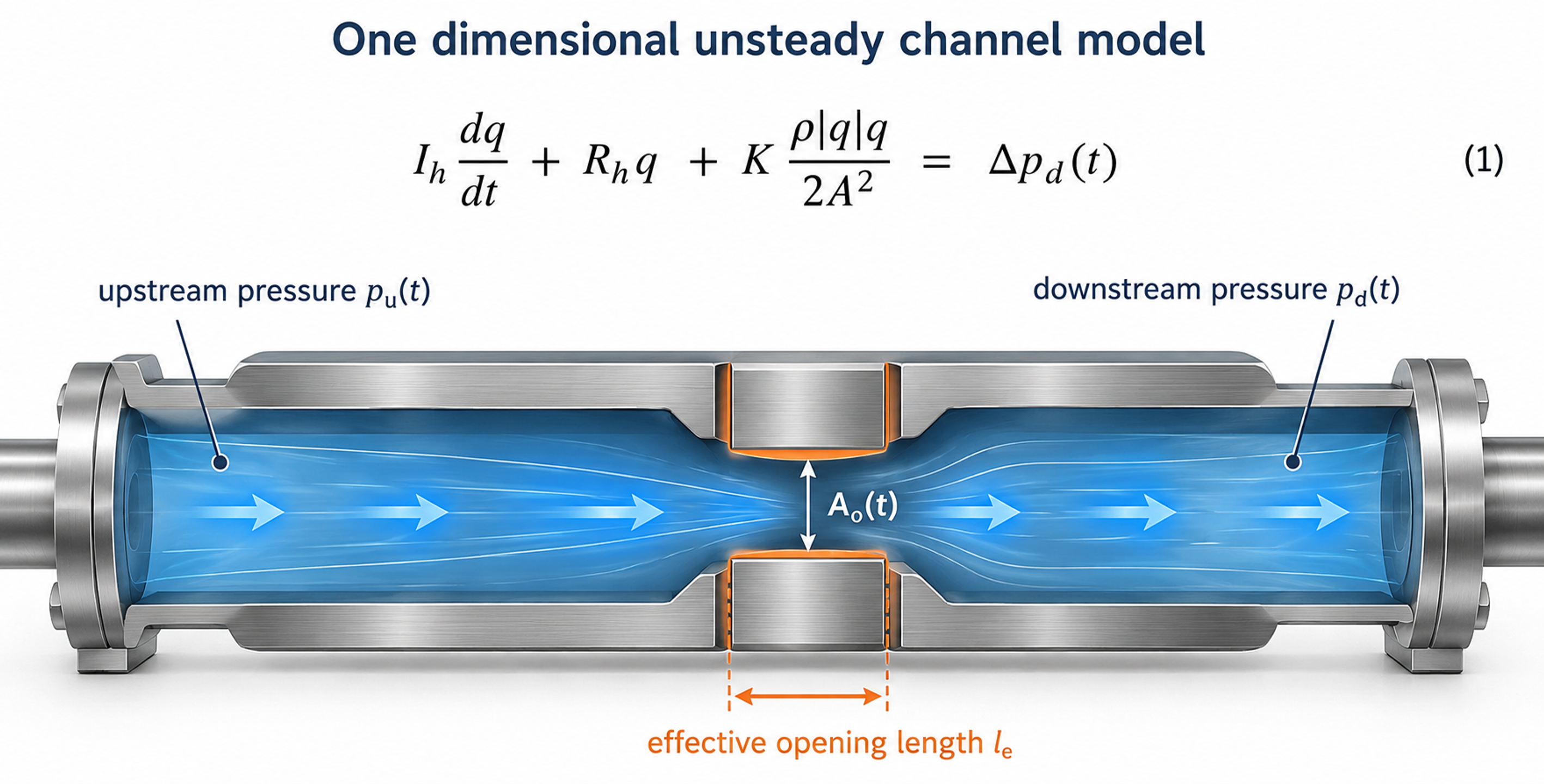
Figure 5.1. Control volume and lumped hydraulic representation of one working passage. The inlet and outlet pressures, effective opening and liquid column length define the model boundary. Diagram based on [1, 8, 13].

5.3 Time varying orifice relation

If the opening behaves as an orifice, the upstream pressure exceeds the downstream pressure, and reverse flow is absent, the instantaneous discharge has the quasi steady approximation

Equation (5.7) applies when the discharge adjusts rapidly relative to the opening period. Significant liquid inertia, rapid area variation, cavitation, or interaction with pressure waves can invalidate this approximation. An improved preliminary model uses Equation (5.7) to express the pressure loss across the restriction and includes that loss once in Equation (5.4). The inertance term then determines the acceleration and phase of the flow. Imposing the full quasi steady discharge and the full transient balance independently across the same pressure difference would overconstrain the model and can count the restriction loss twice.

For a liquid column represented by an effective length, the pressure required for temporal acceleration is estimated by

For an abrupt velocity change in an ideal one dimensional liquid column, the Joukowsky relation provides a limiting pressure change for the generated wave:

Here, $c$ is the wave speed of the liquid and its compliant containment. Application of Equation (5.9) requires a justified velocity change and a closure time short relative to the relevant acoustic travel time. Rotor stator passages usually retain leakage and distributed flow paths, while entrained gas and structural compliance alter the wave speed. Reflections and wave superposition can also change subsequent pressure maxima. The relation is consequently a transient reference estimate, rather than a universal upper bound for every pressure peak in a connected mixing system.

5.4 Dimensionless measures of unsteady flow

The Reynolds number compares convective inertia with viscous transport using a declared reference velocity $U$ and characteristic hydraulic dimension $L$:

The Strouhal number compares the characteristic convective transit time with the period of flow modulation:

The Womersley number expresses the square root of the ratio of oscillatory inertia to viscous diffusion on the selected length scale:

The corresponding penetration depth of an oscillatory viscous boundary layer is

When $\alpha \ll 1$, viscous diffusion acts across the selected length during each cycle, and the velocity profile can adjust closely to the forcing. When $\alpha \gg 1$, an inertia dominated interior and thin oscillatory boundary layers may develop. The length convention must be stated explicitly because use of slot half width, full gap width, or hydraulic radius gives different numerical values. These groups identify relevant transport mechanisms; they do not establish a universal transition criterion for every rotor stator geometry.

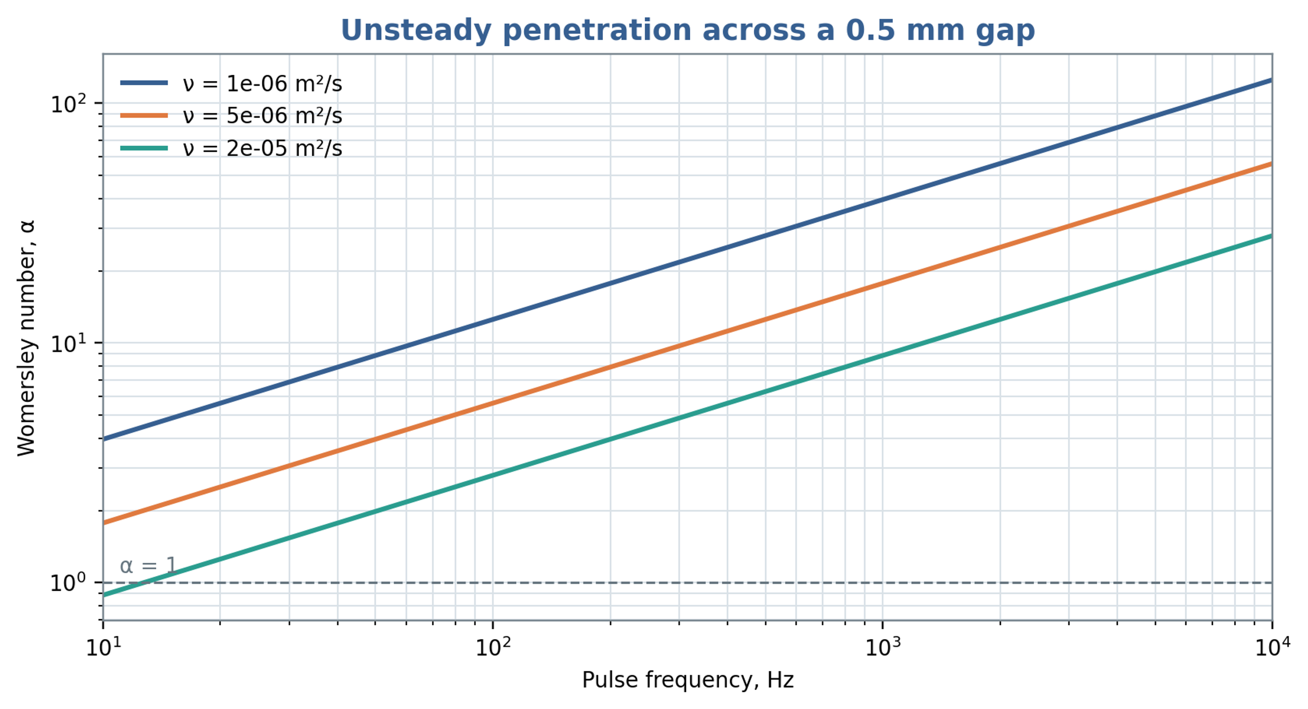
Figure 5.2. Womersley number for a characteristic length of 0.50 mm over pulse frequency and kinematic viscosity, calculated from Equation (5.12).

Table 5.1. Interpretation of principal unsteady flow groups

Group	Small value	Large value	Design consequence
$Re$	Viscous forces dominate	Inertia becomes important; transition depends on geometry	Determines whether laminar resistance or inertial loss is more appropriate
$St$	Slow modulation relative to convection	Rapid modulation	Controls whether a quasi steady or strongly unsteady model is needed
$\alpha$	Velocity profile adjusts through the section during a cycle	Oscillatory boundary layers and phase lag	Important for pulse amplitude and viscous loss
$Eu$	Small pressure change relative to dynamic pressure	Strong restriction or pressure generation	Useful for comparing hydraulic stages

6 Flow in the radial gap

6.1 Cylindrical Couette reference solution

A reference solution for the gap is steady laminar cylindrical Couette flow between an inner cylinder rotating at angular speed $\omega$ and a stationary outer cylinder. For concentric smooth surfaces, no slip, negligible end effects, and no radial or axial throughflow, the tangential velocity is

In the narrow gap limit $\delta \ll R_r$, the tangential velocity profile approaches a linear variation across the clearance. The corresponding nominal shear rate is

For a Newtonian liquid, multiplication by dynamic viscosity gives the nominal viscous shear stress:

The nominal shear rate and stress provide comparison metrics for preliminary screening. Local deformation also includes spatial variations near teeth, slot edges, stagnation regions, recirculation zones, and jets. Partial fluid rotation can reduce the gradient in some regions while increasing it near a stationary surface. The smooth Couette solution can also lose stability to secondary motion as rotational forcing increases. Its applicability therefore depends on the radius ratio, operating regime, end conditions, and throughflow, as well as the nominal gap Reynolds number [14].

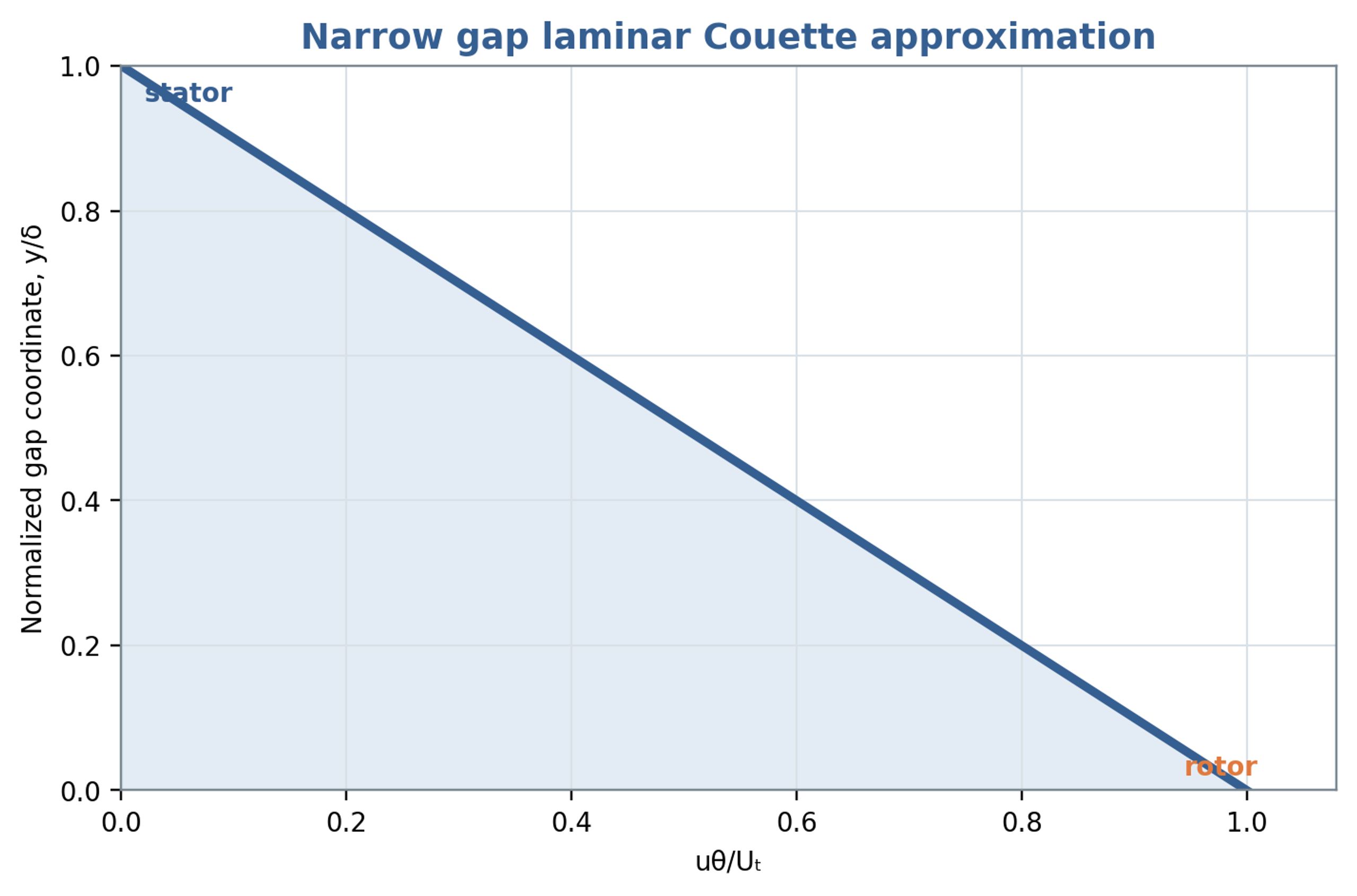
Figure 6.1. Linear tangential velocity profile in the narrow gap Couette approximation, with a moving rotor wall and stationary stator wall.

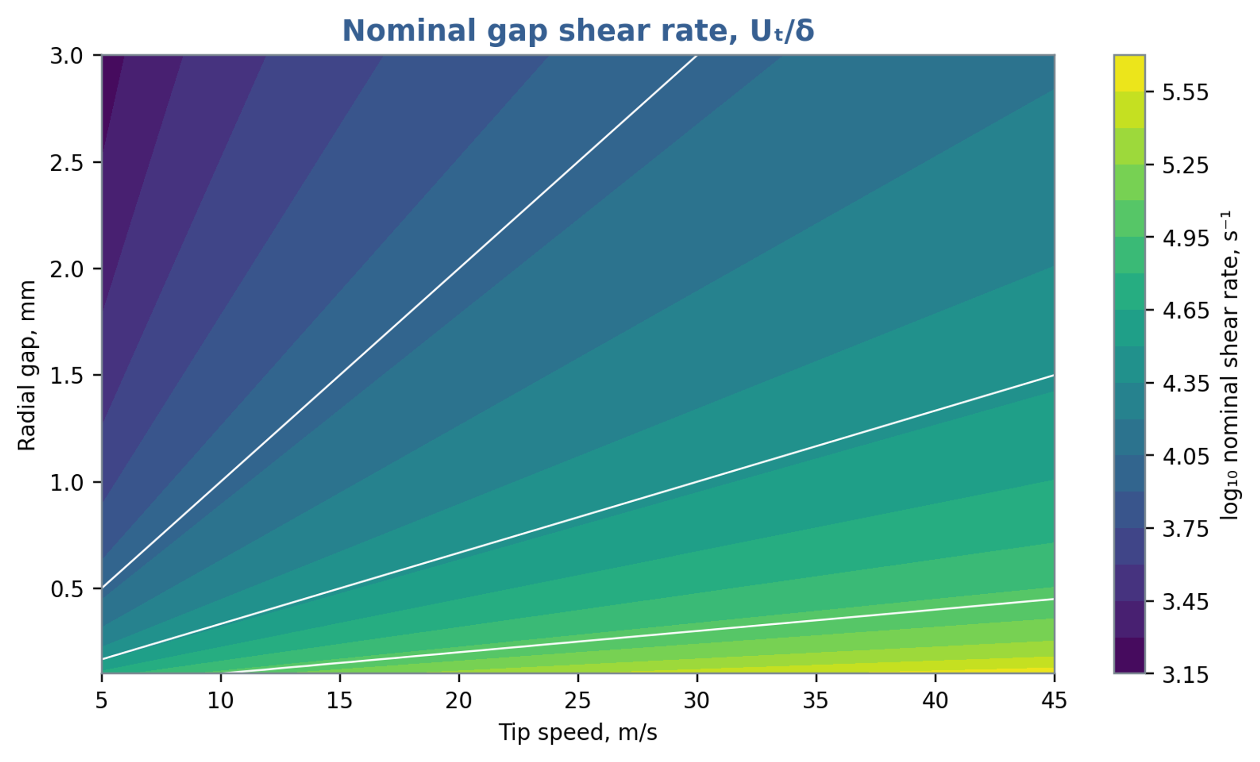
Figure 6.2. Nominal gap shear rate as a function of tip speed and radial clearance, calculated from Equation (6.2). The map represents a geometric screening estimate.

6.2 Gap torque and viscous power

For an inner cylinder with active length $L_g$, integration of the laminar wall shear stress gives the torque magnitude required to maintain its rotation:

The associated rate of viscous energy transfer is

In the narrow gap limit, Equation (6.4) becomes $T_g\approx 2\pi \mu L_g\omega R_r^3/\delta$. The approximation exposes the strong dependence on rotor radius and the inverse dependence on clearance. It is a reference solution for the specified laminar geometry. In a toothed or slotted head, throughflow, secondary circulation, turbulence, roughness, and periodic restriction alter the wall stresses and torque. The result should therefore be used to identify trends and check orders of magnitude, with measured torque providing the final power basis.

Chervyakov and Yudaev develop a broader power balance that separates energy imparted to the flow, viscous losses in radial and axial gaps, and mechanical losses [1]. This decomposition connects power demand to identifiable regions of the apparatus. Because the detailed expressions depend on geometry and flow regime, the present analysis retains the physical structure of the balance and reserves quantitative validation for torque and hydraulic measurements.

6.3 Radial throughflow and pressure

If mean volumetric flow $Q_g$ passes radially through an annular region of active height $H_g$, an average velocity based on the open portion of the circumference is

where ${\varphi }_o$ denotes the effectively open circumferential fraction on the same averaging basis as the flow. During slot passage, the velocity field is spatially nonuniform, with localized jets and pressure gradients in both radial and circumferential directions. Equation (6.6) provides an area based transport estimate and a comparison with the tangential speed. It does not resolve individual jets, local reverse flow, or correlations between instantaneous open area and discharge.

The tangential gap Reynolds number may be formed from $U_t$ and $\delta$, while a throughflow Reynolds number uses $u_r$ and an appropriate hydraulic diameter. Both should be reported when radial transport is substantial. A flow with strong tangential motion and weak radial transport can have a different stress field and residence distribution from a high velocity radial jet at the same rotor tip speed.

6.4 Oscillatory boundary layers and leakage

Passage of a slot can change local radial pressure and velocity over a fraction of a millisecond. At a large gap based Womersley number, rapid viscous adjustment is confined mainly to boundary layers, while the interior responds through inertia. Pressure, flow, and wall stress can consequently exhibit appreciable phase differences. A steady Couette calculation may approximate one contribution to the cycle average while failing to represent the instantaneous torque and stress maxima.

When the principal opening is covered, the remaining clearance provides a leakage path. The minimum effective area consequently helps determine the achievable modulation depth. Increased leakage can weaken pressure pulsation, while a larger mechanical clearance reduces sensitivity to runout and thermal growth. Gap selection should therefore balance deformation rate, pressure modulation, pumping, manufacturing tolerances, erosion, and cleanability within a common hydraulic and mechanical analysis.

7 Hydrodynamic operating parameters

7.1 Throughput and opening area

An engineering velocity scale can be defined using the opening area multiplied by its discharge coefficient:

Equation (7.1) defines a discharge equivalent velocity. The actual mean velocity through a geometric section is the volumetric flow divided by that section area; the discharge coefficient additionally incorporates contraction and velocity losses. Consequently, the equation alone does not determine the physical velocity in the contracted jet. At fixed flow, a smaller simultaneous opening generally increases local velocity, pressure loss, and the likelihood of a pressure minimum. A preliminary screen should evaluate both minimum and mean overlap, while a transient model should use the instantaneous flow and opening together. Unequal flow distribution can produce individual jets substantially different from the area based estimate.

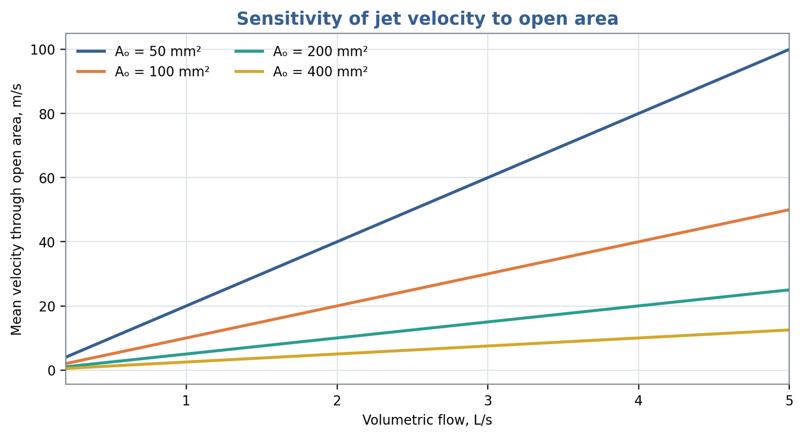
Figure 7.1. Area based mean passage velocity versus throughput for selected opening areas. The calculation uses ${𝐂}_{𝐝}=\mathrm{𝟏}$ in Equation (7.1), so the curves represent geometric section velocities.

7.2 Dimensionless pressure, flow and power

A pressure based Euler number is defined here without a factor of one half in the denominator:

For comparison using turbomachinery similarity, the dimensionless flow coefficient is

The corresponding pressure coefficient is

The power number based on shaft power is

Seminskyi and Vasylenko proposed Euler and Reynolds representations based on flow rate for a rotor pulse apparatus with internal recirculation [9]. Such definitions are useful when measured discharge through a specified region provides the most reproducible velocity scale. Comparisons nevertheless require identical conventions for velocity, length, pressure difference, and power. Geometry, flow coefficient, fluid rheology, and mechanical loss treatment should accompany any reported power number. A coefficient obtained with one set of definitions cannot be transferred quantitatively after those definitions have changed.

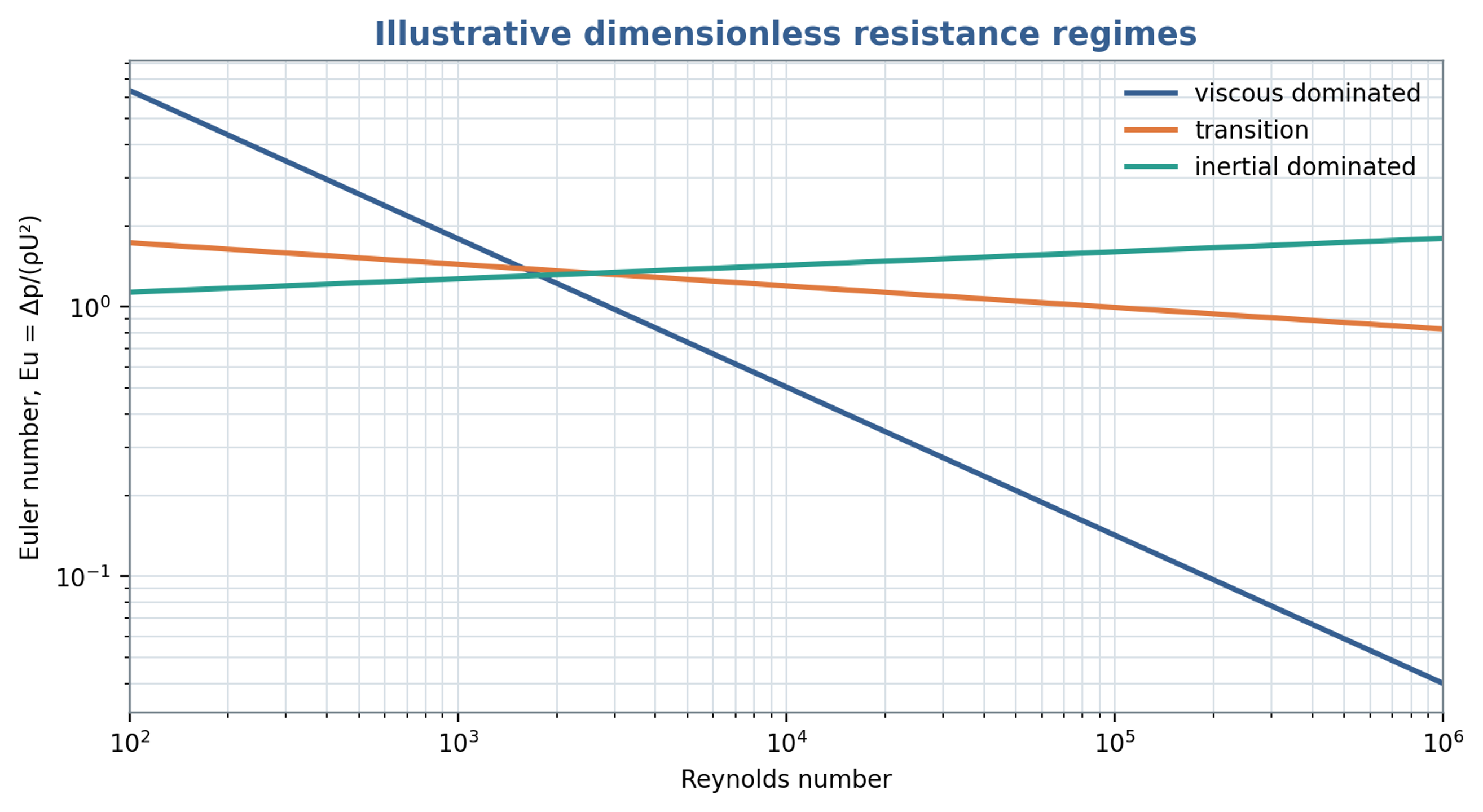
Figure 7.2. Illustrative viscous, transitional and inertial resistance trends. The curves are schematic comparisons and do not constitute fitted universal rotor stator correlations.

7.3 Residence time and nominal event count

For an active internal liquid volume $V_a$ and a representative mean discharge, the nominal residence time is

If $f_p$ denotes the representative local pulse frequency, a nominal event count during one traversal is

The event count $N_p$ is a screening estimate based on nominal residence and a selected frequency. Recirculation, bypassing, gas occupancy, and three dimensional trajectories produce a distribution of exposure histories. A frequency measured by a stationary sensor also need not coincide with the frequency experienced along every moving fluid trajectory. The estimate remains useful for comparing stage volume, discharge, and periodic forcing, provided it is not interpreted as an identical event count for every element of liquid.

7.4 Experimental trends in a single stage apparatus

Seminskyi and Kolobashkin investigated a single stage rotor pulse apparatus with a rotor diameter of 130 mm, 45 rotor slots, a radial clearance of 0.1 mm, a nominal rotational frequency of 50 $s^{-1}$, and a drive rated at 2.2 kW [10]. Within the tested water system, the reported dependencies were consistent with $Q\sim n$, $\mathrm{\Delta }p\sim n^2$, and $P\sim n^3$. These trends resemble centrifugal machine similarity under comparable operating conditions. The reported hydraulic power contribution was no greater than approximately 4 percent for that apparatus. This value pertains to its particular geometry, test circuit, and definition of power. It indicates substantial internal fluid dissipation and mechanical losses while sufficient pressure head remained available to circulate the liquid.

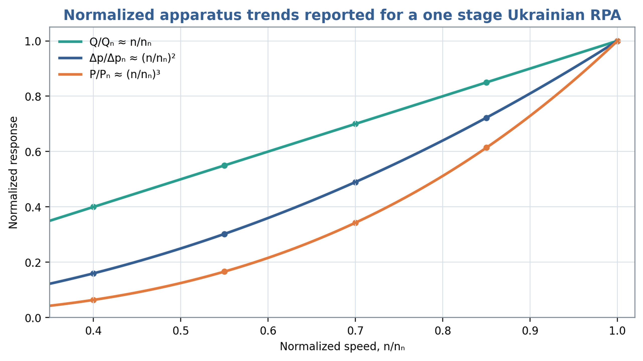
Figure 7.3. Normalized flow, pressure and power trends reconstructed from the proportional dependencies reported for the investigated single stage apparatus. The curves illustrate linear, quadratic and cubic speed scaling, respectively, rather than digitized experimental points [10].

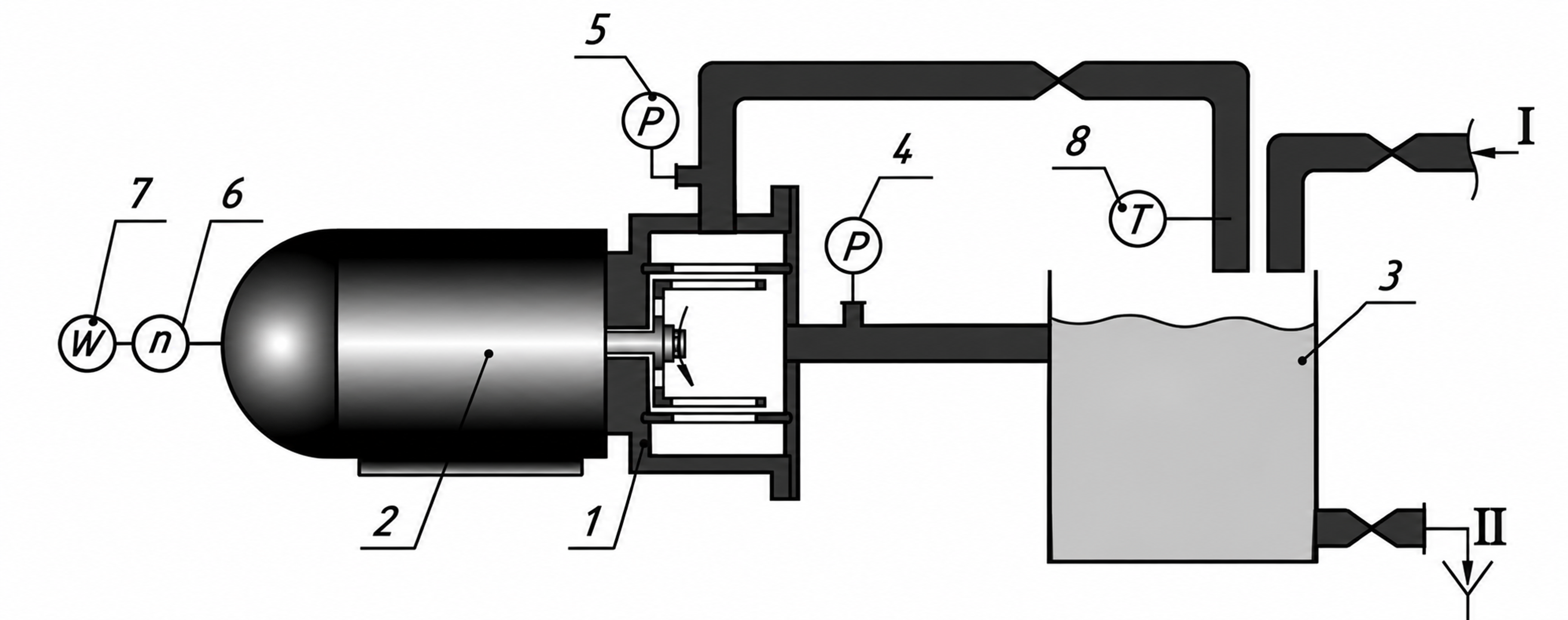
Figure 7.4. Experimental recirculation circuit used by Seminskyi and Kolobashkin [10]. Components: 1, pulsation module; 2, motor; 3, tank; 4, vacuum gauge; 5, pressure gauge; 6, tachometer; 7, wattmeter; 8, thermometer. Connections I and II indicate feed and drainage.

Table 7.1. Reported parameters of the one stage Ukrainian test apparatus [10]

Parameter	Reported value
Rotor diameter	130 mm
Rotor slots	45
Area of one slot	124.5 mm²
Axial perforation area	150.3 mm²
Radial gap	0.1 mm
Maximum volumetric flow	$1.16\times {10}^{-3}$ m³/s
Nominal rotational frequency	50 $s^{-1}$
Nominal drive power	2.2 kW

7.5 Batch circulation and imposed inline flow

External throughput and internal exchange through the stator represent different flow quantities. John et al. combined computational predictions with torque measurements to compare batch and inline operation of a common workhead. Their power and flow characterization accounted for recirculation through the stator openings as well as imposed pipeline flow. This distinction matters when a small net throughput coexists with repeated exchange inside the head. A common characterization was obtained under a restriction on the batch inlet geometry that prevented outward discharge through the base. Therefore, matching external throughput or specific shaft energy alone does not establish equivalent local exposure, droplet histories or pressure pulsations between the two operating modes [15].

8 Pressure pulse energy and cavitation

8.1 Hydraulic specific work

For an incompressible liquid, a pressure difference $\mathrm{\Delta }{p}_p$ defines the hydraulic work scale per unit mass:

The resulting quantity has units of joules per kilogram and represents reversible pressure work for the stated pressure difference. Net energy transfer by an oscillating pressure field additionally depends on the displaced volume and its phase relative to pressure. A large pressure amplitude over a brief event can therefore correspond to little integrated work, while a smaller amplitude sustained over a larger displaced volume can transfer more energy. Hydraulic pressure work and stored wave energy require separate definitions.

Promtov developed calculation approaches for rotary impulse cavitation apparatus using specific measures of pressure pulses, pulsation, and cumulative action [8]. Application of these concepts requires explicit definitions of the integration interval, reference mass, and measured or modeled pressure and flow signals. A pressure amplitude has units of pressure and becomes an energy metric only through a stated physical conversion.

8.2 Acoustic energy and intensity

For a linear progressive plane wave in a uniform liquid, the cycle averaged total acoustic energy density, including kinetic and compressive contributions, is

Dividing that energy density by the liquid density gives the corresponding acoustic energy per unit mass:

Under the same progressive plane wave assumptions, the cycle averaged acoustic intensity is

Equations (8.2) to (8.4) use the root mean square pressure fluctuation. In a progressive plane wave, kinetic and compressive potential energy make equal contributions to the total energy density in Equation (8.2); compressive potential energy alone is half that total. The relations assume linear acoustics and the plane wave pressure to velocity relation. Close to a turbulent or cavitating workhead, reactive pressure fluctuations, standing waves, and multiphase effects can violate those conditions. The equations therefore provide reference wave measures, while local energy transfer requires the appropriate pressure and velocity field [16].

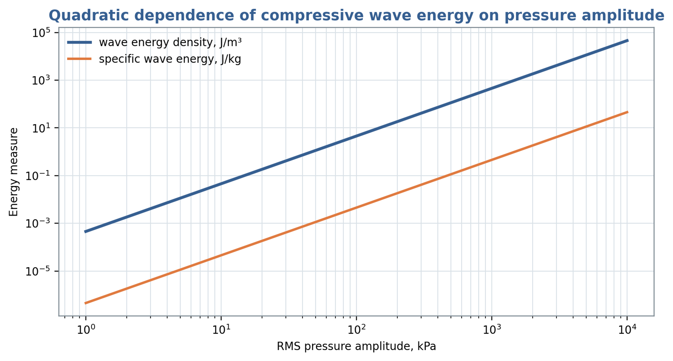
Figure 8.1. Total traveling wave energy per volume and per mass as functions of root mean square pressure amplitude, using Equations (8.2) and (8.3). The retained title refers to compressive energy; the plotted total includes equal kinetic and compressive contributions.

Table 8.1. Pressure related quantities that should not be confused

Quantity	Equation or definition	Units	Meaning
Pressure amplitude	$p_a$ or $p_{rms}^{\prime }$	Pa	Magnitude of fluctuation
Hydraulic specific work	$\mathrm{\Delta }p/\rho$	J/kg	Work associated with a pressure change
Total acoustic wave energy density	$p_{rms}^{\prime 2}/\left(\rho c^2\right)$	J/m³	Cycle averaged kinetic and compressive energy of a linear progressive plane wave
Acoustic intensity	$p_{rms}^{\prime 2}/(\rho c)$	W/m²	Cycle averaged energy flux of a linear progressive plane wave
Hydraulic power	$Q\mathrm{\Delta }p$	W	Product of mean flow and mean pressure difference; omits fluctuation covariance
Pulse fluence	$\int I_{a}dt$	J/m²	Time integrated wave energy per area

8.3 Cavitation number and minimum pressure

A commonly used cavitation number compares the available absolute pressure margin with a reference dynamic pressure:

Here, $p_{ref}$ is absolute pressure at a specified reference location, and $p_v$ is vapor pressure at the local liquid temperature. A smaller $\sigma$ indicates a smaller pressure margin relative to the chosen dynamic pressure. USACE guidance uses cavitation indices for hydraulic screening [17]. Rotating cavitation generators use related definitions, but inception depends on geometry, the velocity convention, nuclei, and the pressure history [18, 19]. A threshold measured for one apparatus should therefore be transferred only with evidence that these conditions are comparable.

A preliminary estimate of the minimum pressure can separate a mean local pressure depression from the negative part of a superimposed pulse:

Cavitation becomes possible as $p_{\text{min}}$ approaches vapor pressure, although nuclei and the duration of the pressure depression influence observable inception. In Equation (8.6), $C_p$ is defined as the positive magnitude of a geometry dependent pressure depression; its sign convention differs from the conventional signed local pressure coefficient. The quantity $p_a$ is the positive magnitude of the additional negative pulse. The steady and oscillatory contributions must be defined consistently to avoid counting the same pressure depression twice. A conservative estimate requires justified coefficients and a credible coincidence of their adverse contributions.

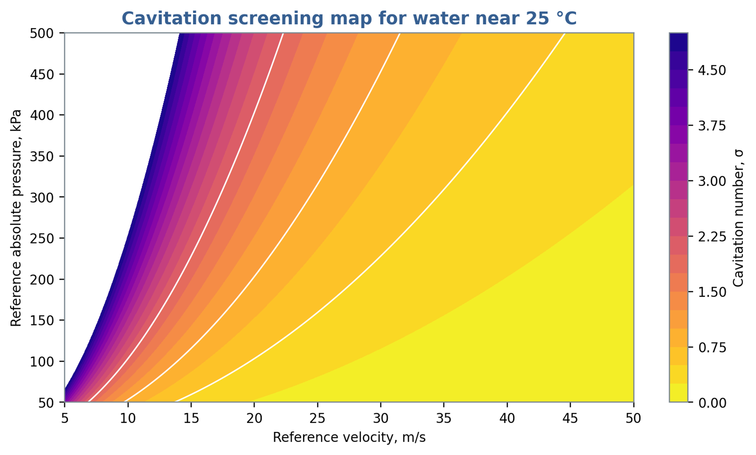
Figure 8.2. Cavitation number calculated from Equation (8.5) using a vapor pressure of 3.2 kPa, representative of water near 25 °C. Pressure is absolute. The contours do not define a universal cavitation inception threshold.

8.4 Bubble dynamics and collapse scales

For an isolated spherical bubble in an effectively infinite incompressible Newtonian liquid, with uniform internal pressure, the Rayleigh Plesset equation describes radial motion:

The symbols $R$, $p_B$, $p_{\infty }$, and $\gamma$ denote bubble radius, internal bubble pressure, imposed far field liquid pressure, and surface tension, respectively [19, 20, 21]. A calculation requires the complete external pressure history, initial radius and wall velocity, and a closure for the gas and vapor pressure inside the bubble. Gas content, thermal response, viscosity, and surface tension influence growth and collapse. Liquid compressibility, strong deformation, and nearby boundaries require more detailed models when their effects are appreciable [19].

For a spherical vapor cavity collapsing from rest under a constant positive pressure difference $p_{\infty }-p_v$, with gas cushioning, viscosity, surface tension, and liquid compressibility neglected, the ideal Rayleigh collapse time is

The product of the maximum cavity volume and its collapse driving pressure gives a characteristic pressure work scale:

Equation (8.9) estimates a cavity energy scale rather than a universal bound on useful treatment energy. Its conversion into sound, rebound, liquid motion, heat, deformation, and viscous dissipation depends on the collapse conditions. Nearby solid surfaces promote asymmetric collapse and can direct a liquid microjet toward the material, producing erosion [19]. Dense clouds introduce interactions and shielding that cannot be represented by a set of independent spherical bubbles without additional coupling. These limitations should accompany any conversion from bubble size to process performance.

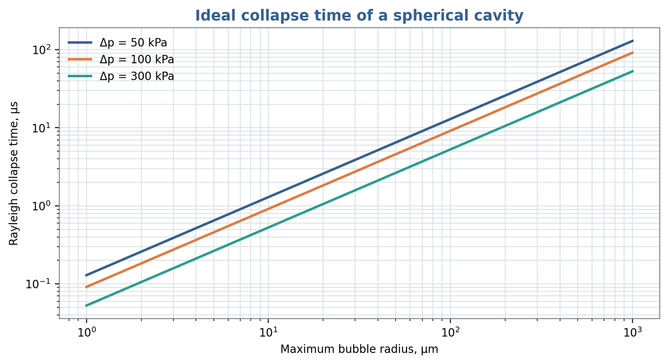
Figure 8.3. Ideal Rayleigh collapse time versus maximum cavity radius and imposed pressure difference, calculated from Equation (8.8). The model neglects gas cushioning, viscosity, surface tension and liquid compressibility.

8.5 Cumulative exposure and process response

A useful cumulative exposure metric should retain pressure amplitude, event duration, event count, and the processed mass. Possible empirical measures include time integrated exposure below a declared pressure threshold or a calibrated acoustic measure within a selected frequency band, referenced to a comparable noncavitating baseline. Product response can then be assessed against exposure, specific shaft energy, and pass count. These metrics require experimental calibration because pressure fluctuations and acoustic emissions do not uniquely determine chemical, biological, or particle response. Nuclei, gas content, reaction kinetics, and device geometry remain relevant explanatory variables.

Promtov and Akulin associated heat generation in a rotor impulse apparatus with cavitation and pressure pulse processes [22]. Assessment of that interpretation requires a complete energy balance. In a closed system, mechanical energy dissipated through shear, turbulence, restriction losses, or bubble motion ultimately contributes to heating, subject to heat removal and energy exported from the boundary. A measured temperature rise therefore quantifies retained thermal energy but does not, by itself, establish which intermediate mechanism dominated.

8.6 Relation to droplet breakup

A product response should accompany hydraulic and power calculations when the objective is emulsification. Hall et al. investigated silicone oil emulsions over a broad range of dispersed phase viscosities in an inline mixer. Rotor speed and dispersed phase viscosity strongly influenced mean droplet size, whereas flow rate had a weaker effect within the tested range. Their interpretation distinguished droplets mainly affected by turbulent inertial stresses from smaller droplets for which viscous effects also became relevant. These observations support specifying formulation properties and the required droplet size distribution alongside nominal gap shear and specific energy. The published trends apply to the investigated formulations and operating conditions and do not define a universal throughput optimum [23].

The location and duration of intense stress influence the interpretation of nominal residence time. Håkansson et al. compared turbulent stress estimates derived from particle image velocimetry with visual observations of droplet breakup. They identified intense regions associated with flow entering a stator hole, the shear layers of the exiting jet and a larger structure produced after rotor blockage. The predicted region near the hole exit agreed with observed breakup locations, although mean stress estimates did not explain every event. This evidence supports interpreting the mixer as a spatially and temporally varying stress field. A nominal pulse count or average residence time should therefore be reported as an exposure descriptor rather than a direct measure of successful fragmentation [24].

9 Power consumption and thermal balance

9.1 Shaft power from torque

Shaft power at a defined measurement location is obtained directly from torque and angular speed:

Converting electrical input to shaft power requires motor and drive efficiencies at the operating load. A suitable baseline over the speed and temperature range is also needed to estimate bearing, seal, and windage contributions. The baseline procedure must preserve the lubrication and cooling conditions required by the apparatus. Incremental torque with liquid present includes hydraulic transport and dissipation associated with gaps, passages, turbulence, and any cavitation. The reported power should identify the measurement plane and state which losses have been subtracted.

9.2 Hydraulic power and efficiency

For mean volumetric flow $Q$ and a pressure rise $\mathrm{\Delta }p$ across the selected boundary, the pressure based hydraulic power is

Using the same operating point and shaft power basis, the hydraulic efficiency is

The hydraulic efficiency ${\eta }_h$ measures the fraction of shaft power represented by the specified pressure rise and circulation flow. Process performance can remain favorable when this fraction is small because internal dissipation may supply the required deformation and dispersion. If inlet and outlet velocities or elevations differ appreciably, the associated kinetic and potential energy changes must also be included in a complete mechanical energy balance. Hydraulic efficiency and product conversion efficiency should consequently be reported as distinct performance measures.

In unsteady operation, pressure and discharge correlations contribute to the cycle averaged hydraulic work. In the following expression, pressure denotes the pressure difference across the chosen boundary, the overbar denotes a cycle average, and primes denote deviations from that average:

For sinusoidal fluctuations with peak amplitudes $p_a$ and $q_a$ and phase difference $\phi$, the oscillatory contribution is $p_a{q}_a\text{cos}\phi /2$. The contribution can be positive, negative, or zero depending on phase. Pressure and flow must therefore be acquired synchronously with known sensor amplitude and phase response. A product of separately averaged signals omits this correlated component.

9.3 Specific energy

For a single pass inline process at steady mean power and throughput, the volumetric and mass specific energy inputs are

The volumetric quantity $E_V$ has units of J/m³, dimensionally equivalent to Pa, whereas $E_m$ has units of J/kg. These measures combine power and throughput and can therefore support comparisons that elapsed processing time alone cannot provide. Their interpretation depends on whether power is gross shaft power or power corrected for mechanical losses. Equal specific energy does not establish equal local stress, exposure distribution, pressure history, or product response.

For a recirculating batch with volume $V_T$ processed for a duration $t$, the gross volumetric energy input at constant or time averaged shaft power is

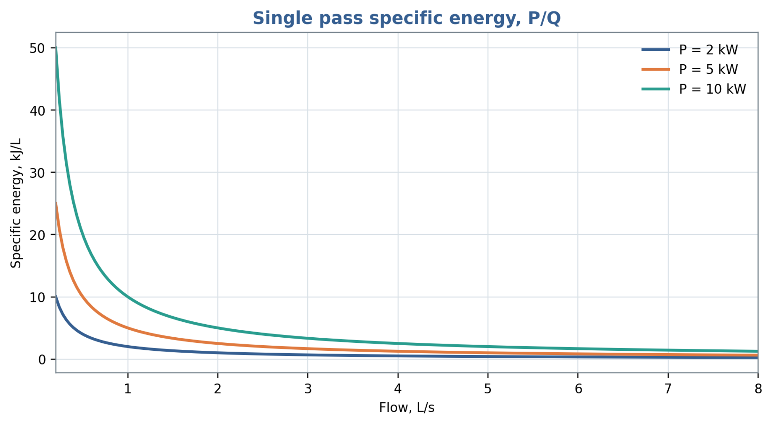
Figure 9.1. Single pass volumetric specific energy as a function of throughput at fixed shaft power, using Equation (9.5). The plotted unit kJ/L is energy per volume; energy per mass additionally requires division by density.

9.4 Heat generation

For a well mixed batch of mass $m$, with approximately constant heat capacity and a fraction ${\eta }_{th}$ of shaft power retained as sensible heat, the temperature rise rate is

For an inline unit, the corresponding temperature rise estimate is $\mathrm{\Delta }T={\eta }_{th}{P}_s/\left(\dot{m}{c}_p\right)$, where the denominator contains mass flow rate and specific heat capacity. The retained thermal fraction depends on the selected boundary and on energy remaining as pressure or motion. Heat removal through the housing, piping, and heat exchanger, as well as heat stored in the equipment, should be included when relevant. Inlet and outlet temperature measurements provide an independent energy balance check when thermal lag, calibration uncertainty, and heat loss are characterized.

For the batch illustrated in Figure 9.2, the retained heating fraction is 0.85 and the assumed constant heat capacity is 4180 J/(kg K). At 30 s, shaft powers of 2, 5 and 10 kW give temperature increases of 0.122, 0.305 and 0.610 °C, respectively. These values establish the seconds time scale of the plotted curves. Over 30 min the corresponding constant property estimates would be 7.32, 18.30 and 36.60 °C; such longer exposure also requires assessment of heat loss and changes in fluid properties.

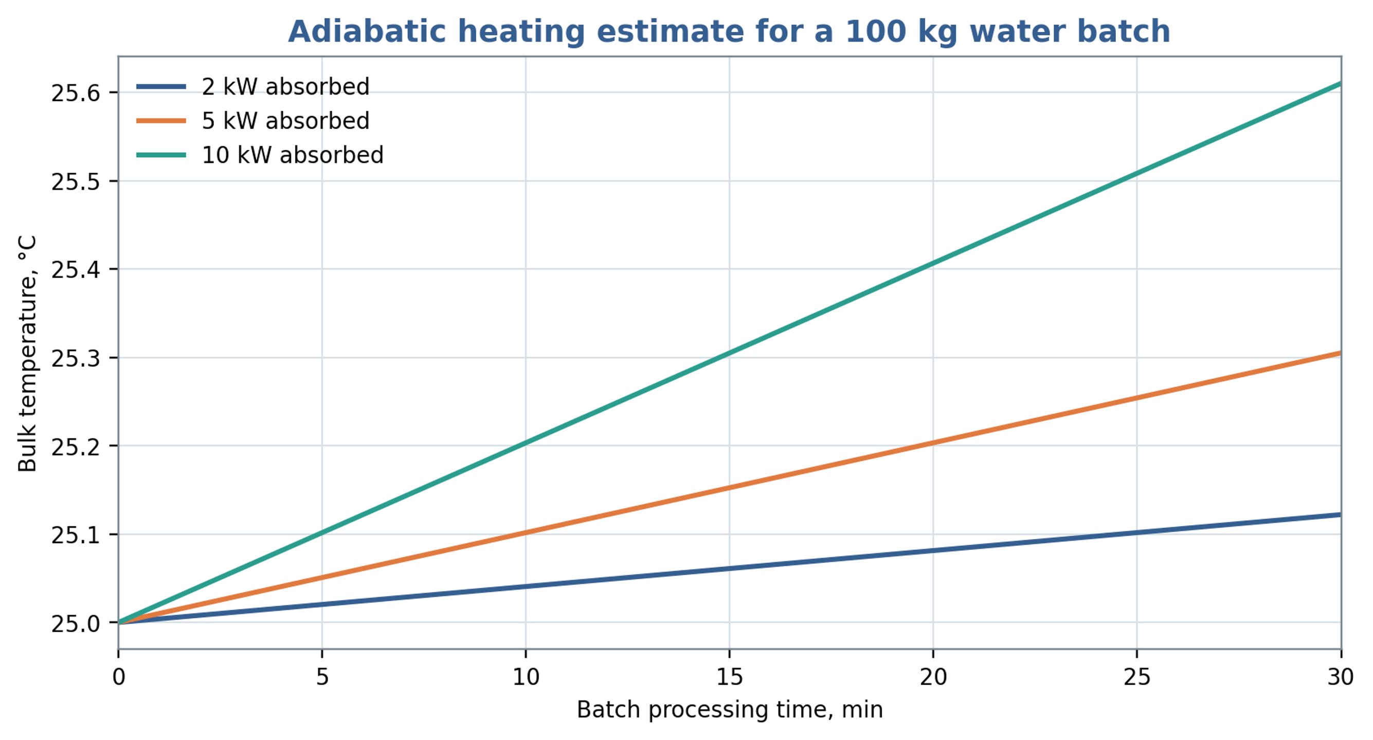
Figure 9.2. Illustrative heating of a 100 kg water batch initially at 25 °C, using Equation (9.7), a heat capacity of 4180 J/(kg K) and ${𝛈}_{𝐭𝐡}=\mathrm{𝟎.𝟖𝟓}$. The plotted time coordinate is in seconds; the embedded min label is incorrect. The legend values are shaft powers before application of the thermal fraction.

9.5 Allocation of power components

A diagnostic allocation of shaft power among hydraulic transport, fluid dissipation, and mechanical loss can be written as

Equation (9.8) provides an accounting structure whose terms must be assigned mutually exclusive physical meanings before they are added. Slot pressure losses already include dissipation caused by jets and turbulence, and cavitation modifies several of those same mechanisms. Adding independently estimated total slot loss, total turbulent dissipation, and total cavitation loss would therefore double count energy. A consistent analysis may allocate losses to separate control volumes or define residual contributions after the directly measured terms are removed. Chervyakov and Yudaev use a related decomposition involving flow kinetic energy, radial and axial gap dissipation, and mechanical loss [1]. Measured shaft power constrains the complete balance.

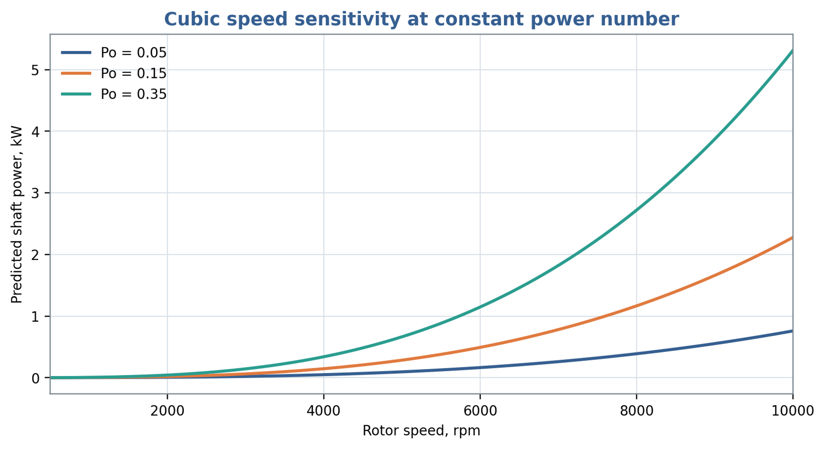
Figure 9.3. Shaft power predicted for selected assumed power numbers using Equation (7.5), $𝐃=\mathrm{𝟖𝟎}$ mm and a density of 1000 kg/m³. These curves illustrate sensitivity to the coefficient and are not validated power predictions for the worked example.

Table 9.1. Power measurements and deductions

Measurement	Directly obtained	Derived quantity	Common error
Shaft torque and speed	$P_s=T\omega$	Fluid load after no load subtraction	Using motor nameplate power as actual shaft power
Inlet and outlet absolute pressure	$\mathrm{\Delta }p$ and cavitation margin	$Q\mathrm{\Delta }p$, $\sigma$	Using only gauge pressure near vacuum
Flow rate	$Q$ or $\dot{m}$	$P/Q$, residence time, flow coefficient	Ignoring pulsation or calibration fluid
Temperature rise	Sensible heat	Approximate thermal fraction	Ignoring heat loss and sensor lag
Fast pressure and flow	$p^{\prime }(t)$ and $q^{\prime }(t)$	$\overline{p^{\prime }{q}^{\prime }}$, spectra, phase	Unsynchronized sampling or inadequate bandwidth
Electrical input	Drive consumption	Shaft power after efficiency correction	Treating variable frequency drive display as torque calibration

9.6 Experimental determination of power characteristics

Experimental power correlations require a defined measurement boundary. James et al. corrected measured torque for bearing losses and instrument offsets before determining power constants for several batch mixer sizes. Their results distinguish laminar, transitional and fully turbulent operation and show that the constants can depend on both mixer scale and workhead geometry. In particular, changes in flow area and removal of the stator screen altered the power characteristics. Consequently, a coefficient determined for one head should be used with its stated Reynolds number definition, rheological conditions and geometric limits. The reported turbulent torque dependence on rotational speed squared also provides a consistency check when cubic power scaling is assumed [25].

10 Engineering calculation procedure

A preliminary engineering calculation should produce a reproducible operating specification and an explicit plan for validating the quantities that remain uncertain. The following sequence connects the preceding relations to equipment selection and commissioning.

1. State the process objective through a measurable particle, droplet, dissolution, reaction or microbial endpoint, together with allowable temperature, pressure, gas entrainment and material wear.

2. Define the control volume for power, flow and pressure measurements, identifying the working head, housing, recirculation circuit or complete vessel as appropriate.

3. Record the active diameters, feature counts, opening dimensions, radial and axial clearances, number of rows and bypass paths.

4. Determine rotational frequency, angular speed and tip speed using Equations (1.1) to (1.3).

5. Evaluate pitch, manufactured slot area and time dependent overlap using Equations (3.1) to (3.6), distinguishing minimum, mean and maximum simultaneous openings.

6. Identify shaft frequency, local feature passage frequency, geometric overlap periodicity and the harmonics relevant to instrumentation and resonance.

7. Estimate passage and gap velocities, nominal residence time and event count using clearly identified flow areas and active volumes.

8. Select a quasi steady or transient passage model from the expected importance of inertia, oscillatory boundary layers and system compliance.

9. Calculate Reynolds, Strouhal, Womersley and Euler numbers, together with flow, pressure and power coefficients, recording the reference scales used in each definition.

10. Evaluate nominal gap shear, viscous stress and laminar Couette torque, and compare their scale with measured or appropriately calibrated power data.

11. Assess cavitation using absolute reference pressure, vapor pressure at the process temperature, a justified velocity scale and a measured or modeled local pressure history.

12. Calculate shaft and hydraulic power, specific energy and the associated thermal load using one consistent boundary and a declared treatment of mechanical losses.

13. Check operating clearance, runout, bearing and shaft loading, seal limits, vibration, erosion and tolerance to particles under the intended operating conditions.

14. Specify the measurements, calibration, sampling bandwidth, uncertainty assessment and product sampling needed to validate the proposed operating range.

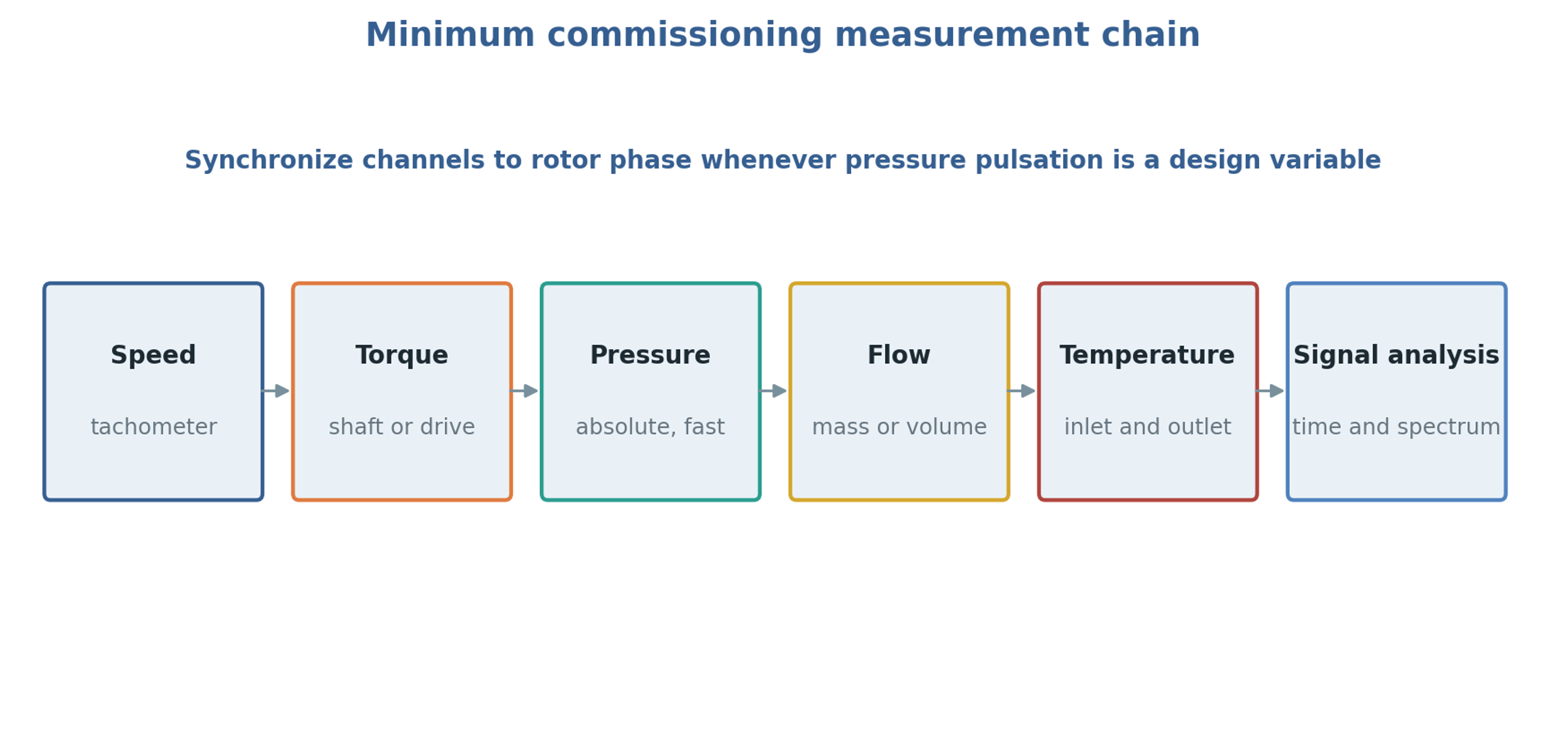
Figure 10.1. Measurement and analysis chain for commissioning. The arrangement represents synchronized acquisition and interpretation of signals rather than a physical sequence of fluid flow.

Table 10.1. Recommended calculation output sheet

Output	Symbol	Unit	Reported basis
Tip speed	$U_t$	m/s	Active outside diameter
Minimum and mean open area	$A_{o,\text{min}}$, ${\overline{A}}_o$	mm²	Specify overlap and leakage area; report discharge coefficient separately
Local pulse frequency	$f_r$	Hz	Rotor feature passage at fixed stator location
Integrated overlap symmetry repeat	$f_A$	Hz	Ideal pattern periodicity or numerical area calculation
Nominal gap shear rate	${\dot{\gamma }}_g$	$s^{-1}$	$U_t/\delta$ screening value
Reynolds, Strouhal, Womersley	$Re$, $St$, $\alpha$	1	Explicit reference length and velocity
Cavitation number	$\sigma$	1	Absolute pressure and local vapor pressure
Shaft power	$P_s$	kW	Measured torque or corrected drive input
Hydraulic power	$P_h$	kW	Mean $Q\mathrm{\Delta }p$ term; report fluctuation covariance separately
Specific energy	$E_m$	kJ/kg	Net or gross basis stated
Temperature rise	$\mathrm{\Delta }T$	°C	Measured and adiabatic estimate

11 Worked screening example

The screening example considers an inline cylindrical stage with the following specified geometry and fluid properties. These inputs define an illustrative Newtonian liquid rather than a complete material specification. In particular, the viscosity is 5 mPa s, so the example should not be interpreted as a pure water calculation at room temperature.

Table 11.1. Specified inputs for the screening example

Input	Value
Rotor outside diameter	80 mm
Shaft speed	6000 rpm
Rotor and stator slots	8 and 12
Radial clearance	0.50 mm
Stator slot width and active height	2.0 mm and 8.0 mm
Mean volumetric flow	2.0 L/s
Liquid density	1000 kg/m³
Dynamic viscosity	5 mPa s
Vapor pressure	3.2 kPa absolute
Reference inlet pressure	200 kPa absolute

The calculated rotational frequency is $N=100$ $s^{-1}$, and the angular speed is 628.3 rad/s. Equation (1.3) gives 25.13 m/s for the tip speed. The rotor passage frequency is 800 Hz from Equation (4.1), whereas the ideal circumferential symmetry repeat is $\text{lcm}(\mathrm{8,12})\times 100=2400$ Hz from Equation (4.2). The latter is a geometric result and does not establish the dominant pressure frequency.

The total manufactured stator opening area is $12\times 2\times 8=192$ mm². Dividing the specified flow by this area gives 10.4 m/s under full exposure with contraction neglected. Rotor opening width has not been specified, so this value does not resolve the minimum simultaneous overlap or the actual contracted jet area. Equation (6.2) gives the nominal gap shear rate as $25.13/(0.0005)=5.03\times {10}^4$ $s^{-1}$, corresponding to approximately 251 Pa for the specified Newtonian viscosity.

Using $U_t$ and the 0.50 mm gap gives a Reynolds number of approximately 2510. At 800 Hz the Womersley number based on the same length is approximately 15.9, indicating that oscillatory inertia and phase lag warrant consideration. Using $U_t$ as the velocity reference in Equation (8.5) gives a cavitation number near 0.62. Cavitation inception cannot be established from this number alone because the local pressure coefficient, pressure fluctuation amplitude and nuclei population are unspecified.

The specified density and viscosity give a kinematic viscosity of 5.0 × 10⁻⁶ m²/s. Equation (5.13) then gives an oscillatory viscous penetration depth of approximately 44.6 µm at 800 Hz, substantially smaller than the 500 µm radial gap. This comparison supports retaining oscillatory inertia in a transient passage calculation. It does not establish a fully turbulent gap state, whose stability and throughflow must be examined separately.

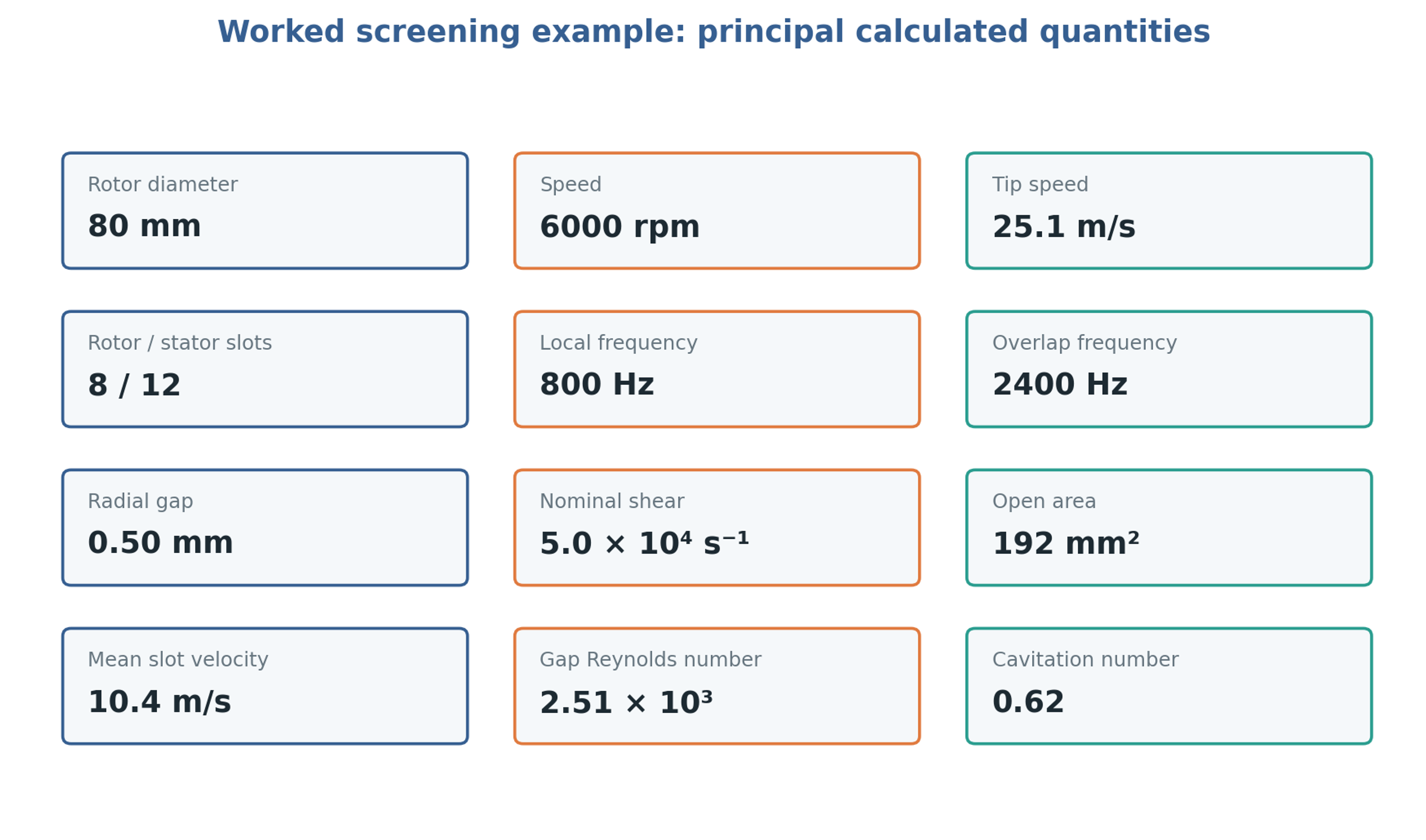
Figure 11.1. Specified and calculated quantities for the screening example. The area is the total geometric stator area and the higher frequency is the ideal overlap symmetry repeat.

Table 11.2. Worked example calculation summary

Quantity	Calculation	Result
Rotational frequency	$6000/60$	100 $s^{-1}$
Tip speed	$\pi (0.08)(6000)/60$	25.13 m/s
Local passage frequency	$8(100)$	800 Hz
Overlap symmetry repeat frequency	$\text{lcm}(\mathrm{8,12})(100)$	2400 Hz
Total geometric stator area	$12(2)(8)$	192 mm²
Nominal slot velocity at full exposure	$0.002/(192\times {10}^{-6})$	10.4 m/s
Nominal gap shear	$25.13/0.0005$	$5.03\times {10}^4$ $s^{-1}$
Nominal shear stress	$0.005(5.03\times {10}^4)$	251 Pa
Gap Reynolds number	$1000(25.13)(0.0005)/0.005$	2510
Cavitation number	$(200-3.2)/\left(0.5(1000){(25.13)}^2/1000\right)$	0.62
Womersley number	Gap based oscillatory inertia measure	15.9
Viscous penetration depth	At the local passage frequency of 800 Hz	44.6 µm

The given inputs do not determine shaft power. A measured torque or a validated power correlation for the actual head is required before specific energy and heat generation can be calculated. Initial characterization should establish mechanical losses with an appropriate safe baseline and then measure the liquid loaded torque over speed and flow. Absolute pressure measurements at the inlet and near the stator discharge are needed to assess the local pressure margin. Representative fluid tests should follow the hydraulic baseline because viscosity and gas content can alter both load and cavitation behavior.

12 Measurement uncertainty and validation

12.1 Torque and speed

Shaft torque provides a direct power basis when speed and transducer calibration are known. The measurement bandwidth should cover the mean load and the torque fluctuations of interest. Mechanical losses should be characterized under comparable speed, temperature and seal conditions. A single constant subtraction is inadequate when bearing or seal friction varies across the operating range. Any baseline procedure must remain compatible with the equipment lubrication and cooling requirements.

12.2 Pressure measurement

Absolute pressure is required for cavitation analysis. Conversion of a gauge signal requires the relevant atmospheric reference. Short, flush pressure ports reduce the filtering and resonance associated with long impulse lines, and trapped gas must be avoided. Sensor bandwidth, sampling frequency and the analog filter used to prevent aliasing should be selected together from the highest pressure harmonic that needs to be resolved. Adequate sample rate cannot recover a fluctuation already attenuated by the pressure port or transducer.

12.3 Flow measurement

An averaged flow signal supports calculation of mean throughput and the mean pressure flow term, but it does not determine the fluctuation product $\overline{p^{\prime }{q}^{\prime }}$. That contribution requires synchronized dynamic pressure and flow measurements with characterized amplitude and phase response. Differential pressure, ultrasonic and other dynamic flow methods require calibration for the installed circuit. Slow changes caused by inventory, gas release or temperature should be distinguished from periodic rotor forcing.

12.4 Temperature and properties

Density, viscosity, vapor pressure, heat capacity and sound speed should correspond to the process temperature and composition. Gas content can strongly affect acoustic response even when its influence on mean density is small. Temperature measurements upstream and downstream of the housing and within the inventory support a thermal balance that includes energy stored in the metal and heat exchanged with the surroundings. Instrument time response must be considered during startup and short processing intervals.

12.5 Spectral and phase analysis

A shaft phase reference permits averaging by rotor position and separates repeatable passage events from broadband fluctuations. Spectral interpretation should distinguish shaft and feature passage components from electrical excitation, structural resonance and broadband turbulence. Increased high frequency noise can accompany cavitation, but it is not unique evidence of cavity formation. Comparison with a noncavitating operating point and simultaneous pressure, vibration and flow measurements improves the interpretation.

Table 12.1. Typical validation questions

Observation	Possible cause	Required check
Pressure peak shifts with flow	Hydraulic phase and changing restriction	Synchronized flow and pressure, system compliance
Shaft power rises faster than $n^3$ in a constant power number regime	Contact, strong viscosity change, choking, or severe cavitation	Hot clearance, temperature, vibration, visual inspection
High frequency noise appears	Cavitation, bearing damage, tooth impact, pipe resonance	Absolute pressure, accelerometers, spectrum, approved mechanical baseline
Flow stops increasing with speed	Choked restriction, gas locking, downstream limit	Open area, pressure, gas fraction, valve position
Temperature rises without expected product change	Energy dissipated outside target mechanism	Power balance, residence distribution, cooling, product sampling
Product response differs at equal $P/Q$	Different local stress, pulse frequency, pressure, or residence distribution	Geometry and spectra, not only gross energy

12.6 Computational verification and model uncertainty

Computational predictions should be evaluated against measurements before local flow features are used for design decisions. In an openly available preprint, Michael et al. compared moving reference frame and sliding mesh treatments, together with alternative turbulence closures, for an inline rotor stator mixer. The sliding mesh treatment better represented transient rotor interactions, while a second moment closure improved flow and power predictions in their comparisons. Appreciable power discrepancies nevertheless remained. The calculation used a simplified two dimensional domain, which limits direct extrapolation to a complete machine. This study illustrates why agreement in integral shaft power does not by itself validate local pressure minima, cavitation intensity or droplet breakup predictions [26].

A numerical validation plan should distinguish numerical error from uncertainty in the physical model. Mesh refinement should resolve the quantities used in the design decision, especially wall gradients, opening jets and pressure minima. Time step refinement should be assessed against the fastest retained passage event. Agreement of mass flow and torque should be checked before interpreting local fields, and sensitivity to inlet conditions, turbulence treatment and any cavitation closure should be reported. A model calibrated at one operating point should be tested at independent combinations of speed, flow and pressure.

12.7 Propagation of measurement uncertainty

Uncertainty should be propagated through the actual calculation rather than attached only to individual instruments. For independent small errors, the relative variance of a product or quotient is obtained by adding the squared relative standard uncertainties, including the exponents of the contributing variables. Correlated errors require covariance terms. Clearance uncertainty deserves particular attention because it directly affects nominal gap shear, while a cavitation number formed from a small pressure margin can be sensitive to errors in both absolute pressure and vapor pressure.

As an illustrative calculation, relative standard uncertainties of 0.5 percent in rotor diameter, 0.5 percent in shaft speed and 4 percent in gap width give approximately 0.71 percent in tip speed and 4.06 percent in nominal gap shear. These assumed values show how clearance can control the combined uncertainty and should be replaced by the actual dimensional and instrument calibration results. Uncertainty in a fitted discharge or power coefficient is additional to measurement uncertainty and must be included when predicting an untested condition.

13 Scale up and design limits

For geometrically similar equipment operating in a comparable flow regime at constant flow, pressure and power coefficients, the standard similarity relations are

These relations require similarity of geometry and operating regime. In practice, clearances, tooth thickness, motor speed and manufacturing tolerance frequently prevent exact geometric scaling. Constant tip speed requires $N\propto D^{-1}$, which changes feature passage frequency if feature count is fixed. Preserving nominal gap shear additionally requires $U_t/\delta$ to remain constant. Matching cavitation number requires a compatible absolute pressure and vapor pressure, while matching specific energy requires coordinated changes in power and throughput. These requirements impose distinct constraints and should be selected according to the process mechanism.

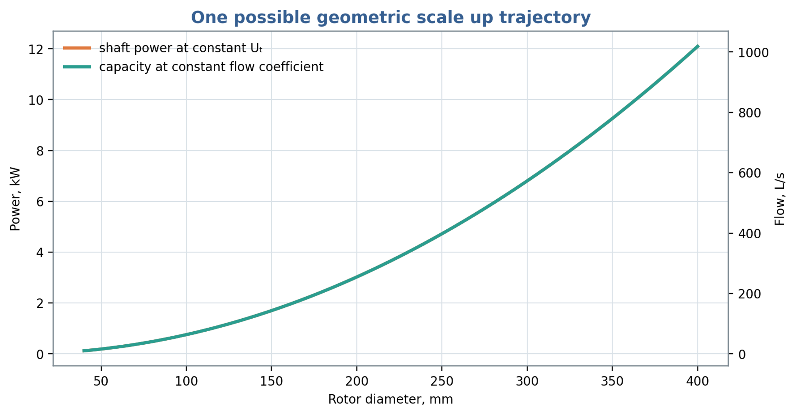
Figure 13.1. Illustrative scaling at constant tip speed, flow coefficient and power number. Under these assumptions, throughput and power both vary with the square of rotor diameter.

Table 13.1. Scale up criteria and quantities preserved

Criterion held constant	Approximately preserves	Does not necessarily preserve
Tip speed	Rotor surface velocity	Pulse frequency, power density, cavitation number
Gap shear $U_t/\delta$	Nominal viscous deformation rate	Turbulence, residence time, opening jets
Power per volume	Mean power input per specified volume	Local peaks, pressure, event frequency
Specific energy $P/(\rho Q)$	Gross energy per processed mass	Stress distribution and thermal history
Cavitation number	Relative pressure margin	Nuclei population, gas content, pulse duration
Flow coefficient	Mean throughput similarity	Slot velocity if open area does not scale
Feature passage frequency	Number of periodic events per time	Tip speed and pumping capacity

13.1 Selection of scaling criteria

Scale selection should follow the required process endpoint. Hall's original doctoral research compared emulsification at three mixer scales and across thirteen rotor and stator configurations. The author reported that tip speed combined with constant residence time was the most suitable basis for correlating mean droplet size across the investigated laboratory and factory equipment, including repeated passes. Stator opening area also affected power and emulsification within a single scale. These findings provide an experimental basis for selecting a practical scaling strategy, while retaining its formulation and geometry limits. Matching this pair of variables does not automatically preserve pulse frequency, gap shear, hydraulic pressure, cavitation margin or temperature rise, which require separate assessment [27].

Table 13.2. Selected experimental and computational evidence relevant to engineering scale up

Study	Quantity investigated	Engineering implication and limit
James et al. [25]	Torque and power constants	Constants depend on the tested workhead and regime; verify corrected torque.
John et al. [15]	Batch and inline circulation	External throughput differs from internal exchange; match the flow definition.
John et al. [12]	Screen and inlet geometry	Controlled geometry changes support calibrated power and flow relations.
Hall et al. [23]	Emulsion droplet size	Formulation and local stresses limit transfer of specific energy correlations.
Håkansson et al. [24]	Local fragmenting stresses	Breakup location depends on the spatial and transient stress field.
Ayas et al. [11]	Viscoplastic liquid mixing	Constitutive behavior and local shear need explicit treatment.
Michael et al. [26]	CFD power and flow	A simplified preprint model retains substantial prediction uncertainty.
Hall [27]	Emulsification across scales	Tip speed with residence time was useful within the investigated systems.

Mechanical and service requirements constrain the hydraulic scaling. Centrifugal stress and shaft deflection can affect the maintained gap; thermal expansion can reduce clearance; and cavitation or abrasive wear can change opening edges and discharge behavior. Cleaning requirements may also impose minimum accessible passage dimensions. Scale up should therefore proceed through hydraulic characterization, representative fluid testing, verification of heat removal and wear, and confirmation of the product endpoint over the intended operating envelope.

13.2 Workhead selection and geometric documentation

The photographs in Figure 13.2 and Figure 13.3 illustrate the range of screen forms that can be fitted around a rotor. Their relevance to engineering calculation lies in the opening dimensions, edge thickness, accessible clearance and inlet arrangement. A screen designation should therefore be accompanied by its measured geometry when comparing power, circulation and product response [28].

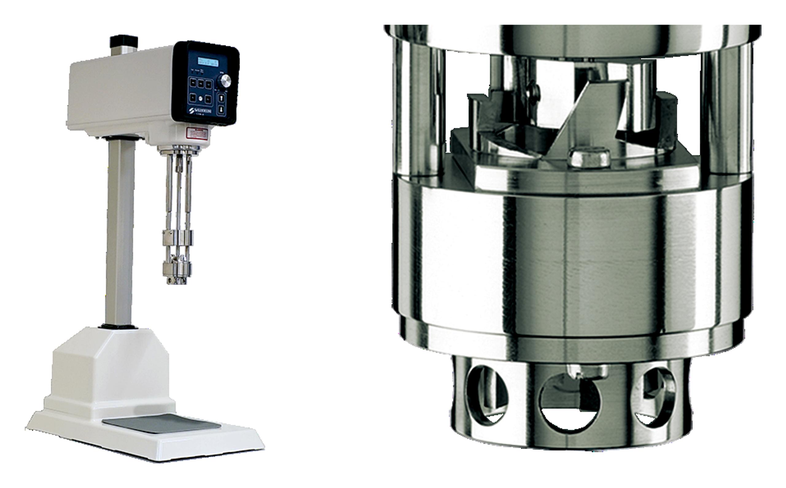
Figure 13.2. Representative laboratory mixer and a close view of its working head. Photographs from Silverson technical literature [28].

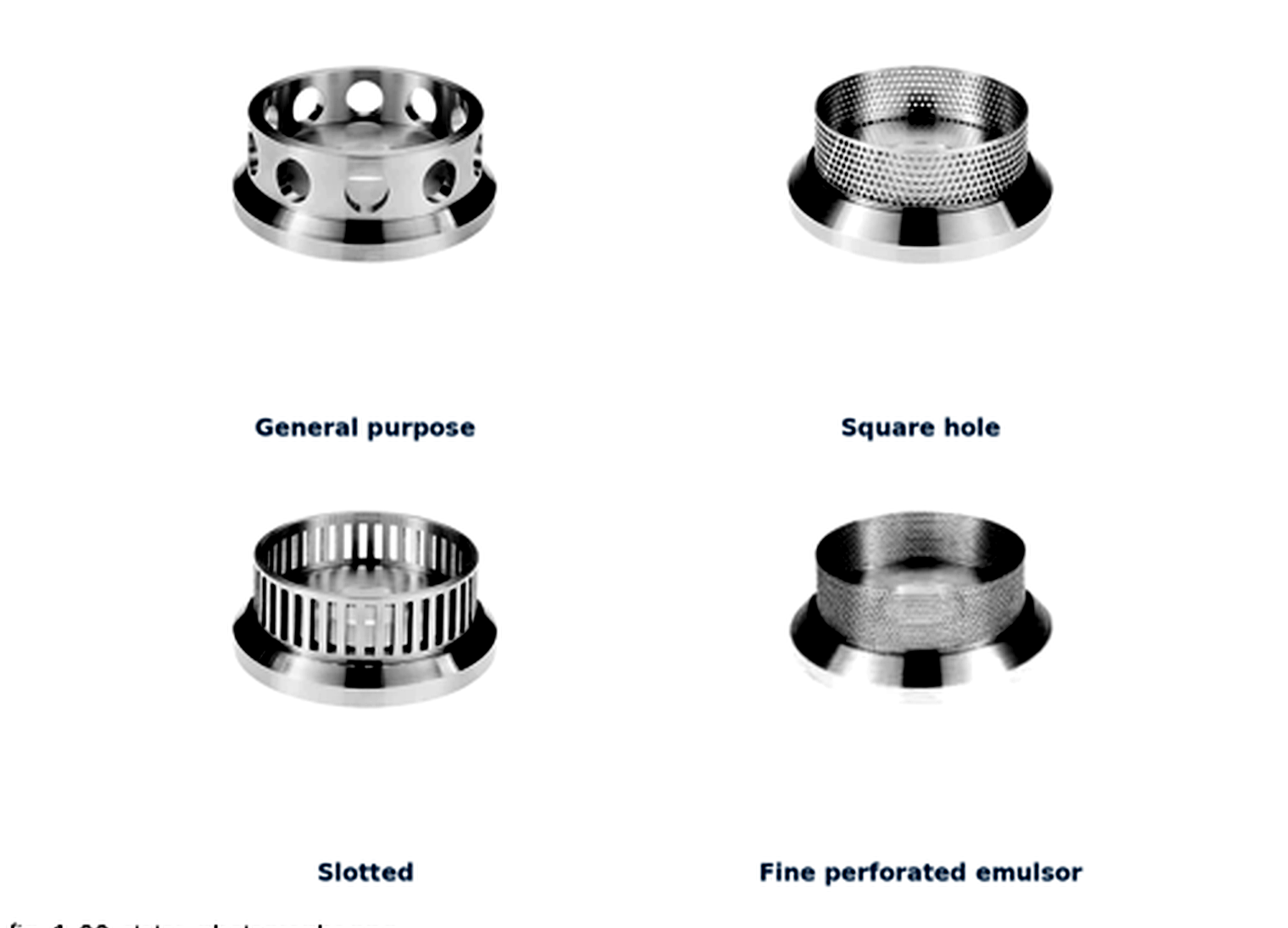
Figure 13.3. Examples of commercial stator screens with general purpose, square hole, slotted and fine perforated configurations. Photographs and screen designations from Silverson technical literature [28].

14 Conclusions

Rotor-stator calculations require explicit geometry and boundary conditions. Diameter and speed establish tip speed, while clearance, opening dimensions, feature count and row arrangement govern exposure, leakage and periodic forcing. Local feature passage frequency and integrated overlap symmetry describe different aspects of the geometry and cannot be substituted for a measured pressure spectrum.

A hierarchy of models provides a practical basis for engineering analysis. The lumped inertance model describes acceleration and hydraulic phase, while Couette flow supplies a reference for viscous gap behavior. The nominal rate $U_t/\delta$ summarizes one velocity gradient but does not resolve the strain and dissipation encountered along actual fluid trajectories. Reynolds, Strouhal and Womersley numbers help identify the limits of these reductions and the measurements needed to test them.

Energy quantities require consistent definitions. Hydraulic work $\mathrm{\Delta }p/\rho$, the traveling wave energy scale $p^{\prime 2}/\left(\rho c^2\right)$, hydraulic power $Q\mathrm{\Delta }p$ and shaft energy per mass $P/(\rho Q)$ describe different transfers and cannot be inferred interchangeably from pressure amplitude. Cavitation assessment further requires absolute pressure, vapor pressure, nuclei and the duration of the low pressure exposure. Isolated spherical bubble models provide useful scales but require additional treatment for wall effects and interacting clouds.

The screening example establishes plausible kinematic, shear and oscillatory scales while leaving shaft power and cavitation inception unresolved by the available inputs. Published experimental and computational studies support the use of geometry specific power and flow characterization, together with product measurements, for scale up. A consistent energy balance must avoid counting the same slot, turbulent or cavitation dissipation more than once. The resulting design basis is strongest when it reports both predicted values and the operating conditions under which they have been validated.

15 Nomenclature

Table 15.1. Latin symbols

Symbol	Definition	SI unit
$A$	Reference flow area	m²
$A_o$	Geometric simultaneous opening area, including stated leakage paths	m²
$A_s$	Total geometric stator slot area	m²
$b_r$, $b_s$	Rotor and stator slot width	m
$c$	Wave speed in liquid or compliant fluid system	m/s
$c_p$	Specific heat capacity	J/(kg K)
$C_d$	Discharge coefficient	1
$C_p$	Positive pressure depression coefficient used in the minimum-pressure screen	1
$D$	Active rotor diameter	m
$e_a$	Total acoustic wave energy per unit mass	J/kg
$e_{p,h}$	Hydraulic specific work of a pressure pulse	J/kg
$E_b$	Characteristic cavity collapse work	J
$E_V$	Volumetric specific energy	J/m³
$f_A$	Integrated overlap symmetry repeat frequency	Hz
$f_p$	Selected pressure or feature passage frequency	Hz
$f_r$	Local rotor feature passage frequency	Hz
$h$	Slot height or small channel dimension	m
$I_a$	Cycle averaged acoustic intensity for a progressive plane wave	W/m²
$I_h$	Hydraulic inertance	kg/m⁴
$K$	Local loss coefficient	1
$L$, $L_g$	Characteristic length or active gap length	m
$l_e$	Effective channel length	m
$m$	Batch mass	kg
$m_A$	Area modulation index	1
$N$	Rotational frequency	$s^{-1}$
$N_p$	Nominal number of pulse events	1
$n$	Rotor speed	rpm
$p$	Pressure; pressure difference in the hydraulic covariance relation	Pa
$p_a$	Peak pressure amplitude; positive negative-pulse magnitude in cavitation screening	Pa
$p_v$	Vapor pressure	Pa
$P_h$	Hydraulic power	W
$P_s$	Shaft power	W
$Po$	Power number	1
$p_r$, $p_s$	Rotor and stator pitch	m
$q$	Instantaneous flow through one modeled passage	m³/s
$Q$	Mean volumetric flow	m³/s
$R$	Bubble radius or generic radius, as defined	m
$R_h$	Linear hydraulic resistance	Pa s/m³
$R_r$, $R_s$	Rotor and stator radii	m
$Re$	Reynolds number	1
$St$	Strouhal number	1
$T$	Torque or temperature, as defined by context	N m or K
$t$	Time	s
$t_a$	Nominal active zone residence time	s
$t_c$	Rayleigh collapse time	s
$t_o$	Nominal opening duration	s
$U$	Reference velocity	m/s
$U_o$	Discharge equivalent velocity based on coefficient times opening area	m/s
$U_t$	Rotor tip speed	m/s
$u_r$, $u_{\theta }$	Radial and tangential velocity components	m/s
$V_a$	Active internal volume	m³
$V_T$	Tank or loop inventory volume	m³
$z_r$, $z_s$	Number of rotor and stator features	1
$A_{o,min},\overline{A_o}$	Minimum and cycle averaged simultaneous opening area	m²
$D_r,D_s$	Active rotor and stator diameters	m
$b_e$	Effective circumferential width defining an exposure event	m
$t_r$	Circumferential rotor tooth or bridge width	m
$h_s$	Stator slot active height	m
$H_g$	Active height of the radial throughflow region	m
$w$	Width of the parallel plate channel	m
$g(\cdot )$	Zero mean periodic overlap shape function	1
$𝐠$	Gravitational acceleration vector	m/s²
$𝐮$	Fluid velocity vector	m/s
$f_s$	Stator passage frequency observed in the rotating frame	Hz
$Q_g$	Mean radial flow crossing the gap on the declared area basis	m³/s
$T_g$	Laminar cylindrical gap torque magnitude	N m
$P_g$	Laminar cylindrical gap power	W
$Eu$	Euler number on the stated pressure and velocity basis	1
$E_m$	Shaft energy input per processed mass	J/kg
$E_{V,b}$	Gross volumetric energy input to a recirculating batch	J/m³
$E_{v,a}$	Cycle averaged total acoustic wave energy density	J/m³
$p_{ref},p_{\text{min}}$	Absolute reference and minimum local pressures	Pa
$p_u,p_d$	Pressures upstream and downstream of the modeled restriction	Pa
$\mathrm{\Delta }{p}_d(t)$	Net time dependent driving pressure in the lumped passage balance	Pa
$\mathrm{\Delta }{p}_p$	Pressure difference used to define hydraulic specific pulse work	Pa
$p_B,p_{\infty }$	Bubble internal pressure and imposed far field liquid pressure	Pa
${p^{\prime }}_{rms}$	Root mean square pressure fluctuation	Pa
$R_{\text{max}}$	Maximum bubble radius at the beginning of ideal collapse	m
$\dot{m}$	Mass flow rate through the inline unit	kg/s
$q_a$	Peak amplitude of sinusoidal flow fluctuation	m³/s
$P_{pump}$	Power exported as hydraulic transport	W
$P_{gap,r}$	Power assigned to the radial gap	W
$P_{gap,a}$	Power assigned to the axial gap	W
$P_{slot}$	Power assigned to passage losses	W
$P_{turb}$	Residual turbulent dissipation not counted elsewhere	W
$P_{cav}$	Residual cavitation related dissipation not counted elsewhere	W
$P_{mech}$	Mechanical loss power within the declared boundary	W

Table 15.2. Greek symbols

Symbol	Definition	SI unit
$\alpha$	Womersley number	1
$\delta$	Radial rotor stator gap	m
${\delta }_{\nu }$	Oscillatory viscous penetration depth	m
$\mathrm{\Delta }p$	Pressure difference	Pa
${\dot{\gamma }}_g$	Nominal gap shear rate	$s^{-1}$
$\gamma$	Surface tension	N/m
${\eta }_h$	Hydraulic efficiency	1
${\eta }_{th}$	Fraction of shaft power retained as sensible heat	1
$\mu$	Dynamic viscosity	Pa s
$\nu$	Kinematic viscosity	m²/s
${\varphi }_A$	Phase of area waveform	rad
${\varphi }_o$	Effective open fraction	1
${\varphi }_Q$	Flow coefficient	1
$\rho$	Density	kg/m³
$\sigma$	Cavitation number	1
${\tau }_g$	Nominal gap shear stress	Pa
$\omega$	Angular speed	rad/s
${\omega }_p$	Angular pressure pulse frequency	rad/s
$\psi$	Head or pressure coefficient	1
$\phi$	Phase difference between pressure and flow fluctuations	rad
${\varphi }_s$	Geometric circumferential stator open fraction	1

Bibliography

[1] Chervyakov VM, Yudaev VF. Gidrodinamicheskie i kavitatsionnye yavleniya v rotornykh apparatakh [Hydrodynamic and cavitation phenomena in rotary apparatus]. Moscow: Mashinostroenie-1; 2007. 128 p. Russian. https://files.znu.edu.ua/files/Bibliobooks/Inshi32/0028381.pdf.

[2] Balabyshko AM, Yudaev VF. Rotornye apparaty s modulyatsiey potoka i ikh primenenie v promyshlennosti [Rotary apparatus with flow modulation and their industrial application]. Moscow: Nedra; 1992. 176 p. Russian.

[3] Balabudkin MA. Rotorno-pulsatsionnye apparaty v khimiko-farmatsevticheskoy promyshlennosti [Rotor pulse apparatus in the chemical and pharmaceutical industry]. Moscow: Meditsina; 1983. 160 p. Russian.

[4] Kremnev OA, Borovsky VR, Lopatin VV, Zhukotsky EK, inventors. Rotor-pulse apparatus. Soviet patent SU829155A1. 1981 May 15. https://patents.google.com/patent/SU829155A1/en.

[5] Ross JC, inventor. Low profile rotors and stators for mixers and emulsifiers. United States patent US5632596A. 1997 May 27. https://patents.google.com/patent/US5632596A/en.

[6] Kozyuk O. Rotor Stator Mixer. [Unpublished technical manuscript and supporting data] 2026.

[7] Promtov MA. Pulsatsionnye apparaty rotornogo tipa: teoriya i praktika [Rotary type pulsation apparatus: theory and practice]. Moscow: Mashinostroenie-1; 2001. 260 p. Russian. https://imptec.ru/publikatsii-i-patenty.

[8] Promtov MA. Foundations of method of calculating rotor impulse-cavitation apparatus. Transactions of Tambov State Technical University. 2004;10(1A):149–154. Russian. https://vestnik.tstu.ru/rus/t_10/pdf/10_1_014.pdf.

[9] Seminskyi OO, Vasylenko RM. Energy parameters of flows in the working members of a rotor pulse apparatus. Bulletin of the National Technical University of Ukraine Kyiv Polytechnic Institute: Chemical Engineering, Ecology and Resource Saving. 2015;1(14):83–85. Ukrainian. https://ela.kpi.ua/bitstreams/1f4167ed-8e45-47bc-8927-710bf9ad4780/download.

[10] Seminskyi OO, Kolobashkin LV. Hydrodynamic characteristics of a single-stage high shear mixer with compensation of axial pressure in the end clearance between rotor and housing. Mechanics and Advanced Technologies. 2017;3(81):69–74. https://doi.org/10.20535/2521-1943.2017.81.119080. Open text.

[11] Ayas M, Skocilas J, Jirout T. Analysis of power input of an in-line rotor-stator mixer for viscoplastic fluids. Processes. 2020;8(8):916. https://doi.org/10.3390/pr8080916. Open text.

[12] John TP, Panesar JS, Kowalski A, Rodgers TL, Fonte CP. Linking power and flow in rotor-stator mixers. Chemical Engineering Science. 2019;207:504–515. https://doi.org/10.1016/j.ces.2019.06.039. Open text.

[13] Promtov MA, Stepanov AYu. Computer system for calculation of a rotary impulse apparatus. Transactions of Tambov State Technical University. 2011;17(1):83–89. Russian. https://vestnik.tstu.ru/rus/t_17/pdf/17_1_010.pdf.

[14] Taylor GI. Stability of a viscous liquid contained between two rotating cylinders. Philosophical Transactions of the Royal Society of London. Series A. 1923;223:289–343. https://doi.org/10.1098/rsta.1923.0008.

[15] John TP, Fonte CP, Kowalski A, Rodgers TL. A comparison of power and flow characteristics between batch and in-line rotor-stator mixers. Chemical Engineering Science. 2019;202:481–490. https://doi.org/10.1016/j.ces.2019.03.015. Open text.

[16] Smith JO III. Physical audio signal processing: for virtual musical instruments and audio effects. W3K Publishing; 2010. Section: Acoustic energy density. https://www.dsprelated.com/freebooks/pasp/Acoustic_Energy_Density.html.

[17] US Army Corps of Engineers. Hydraulic design of reservoir outlet works. Engineer Manual EM 1110-2-1602. Washington, DC: Department of the Army; 1980 Oct 15. Available online.

[18] Omelyanyuk M, Ukolov A, Pakhlyan I, Bukharin N, El Hassan M. Optimization of rotational hydrodynamic cavitation reactor geometry. Fluids. 2024;9(10):244. https://doi.org/10.3390/fluids9100244. Open text.

[19] Brennen CE. Cavitation and bubble dynamics. New York: Oxford University Press; 1995. 294 p. https://media.library.caltech.edu/CaltechBOOK:1995.001/chap2.htm.

[20] Rayleigh, Lord. On the pressure developed in a liquid during the collapse of a spherical cavity. The London, Edinburgh, and Dublin Philosophical Magazine and Journal of Science. 1917;34(200):94–98. https://doi.org/10.1080/14786440808635681. Open text.

[21] Plesset MS. The dynamics of cavitation bubbles. Journal of Applied Mechanics. 1949;16(3):277–282. https://doi.org/10.1115/1.4009975. Open text.

[22] Promtov MA, Akulin VV. Mechanisms of heat generation in a rotary impulse apparatus. Transactions of Tambov State Technical University. 2006;12(2A):364–369. Russian. https://dewa.ru/wp-content/heating-methods-in-ria.pdf.

[23] Hall S, Cooke M, El-Hamouz A, Kowalski AJ. Droplet break-up by in-line Silverson rotor–stator mixer. Chemical Engineering Science. 2011;66(10):2068–2079. https://doi.org/10.1016/j.ces.2011.01.054. Open text.

[24] Håkansson A, Mortensen HH, Andersson R, Innings F. Experimental investigations of turbulent fragmenting stresses in a rotor-stator mixer. Part 1: Estimation of turbulent stresses and comparison to breakup visualizations. Chemical Engineering Science. 2017;171:625–637. https://doi.org/10.1016/j.ces.2017.06.042. Public abstract.

[25] James J, Cooke M, Trinh L, Hou R, Martin P, Kowalski A, Rodgers TL. Scale-up of batch rotor–stator mixers. Part 1: Power constants. Chemical Engineering Research and Design. 2017;124:313–320. https://doi.org/10.1016/j.cherd.2017.06.020. Open text.

[26] Michael V, Ahmed U, Assad M, Prosser R, Kowalski A. Flow characterisation and power consumption in an inline high shear rotor-stator mixer using CFD. arXiv [Preprint]. 2023;2305.16738. https://doi.org/10.48550/arXiv.2305.16738. Open text.

[27] Hall S. Scale-up of emulsification in in-line rotor–stator mixers [EngD thesis]. Birmingham: University of Birmingham; 2013. https://etheses.bham.ac.uk/id/eprint/4045/. Open text.

[28] Silverson Machines. Laboratory scale mixers: high speed high shear mixers. Manufacturer brochure. Undated. Section: Interchangeable heads and screens, p. 4. https://www.silverson.com/images/uploads/documents/Silverson_Brochure_Laboratory_Mixers_US.pdf.