Engineering Calculations for Rotor-Stator Mixers

9 Power consumption and thermal balance

9.1 Shaft power from torque

Shaft power at a defined measurement location is obtained directly from torque and angular speed:

Converting electrical input to shaft power requires motor and drive efficiencies at the operating load. A suitable baseline over the speed and temperature range is also needed to estimate bearing, seal, and windage contributions. The baseline procedure must preserve the lubrication and cooling conditions required by the apparatus. Incremental torque with liquid present includes hydraulic transport and dissipation associated with gaps, passages, turbulence, and any cavitation. The reported power should identify the measurement plane and state which losses have been subtracted.

9.2 Hydraulic power and efficiency

For mean volumetric flow $Q$ and a pressure rise $\mathrm{\Delta }p$ across the selected boundary, the pressure based hydraulic power is

Using the same operating point and shaft power basis, the hydraulic efficiency is

The hydraulic efficiency ${\eta }_h$ measures the fraction of shaft power represented by the specified pressure rise and circulation flow. Process performance can remain favorable when this fraction is small because internal dissipation may supply the required deformation and dispersion. If inlet and outlet velocities or elevations differ appreciably, the associated kinetic and potential energy changes must also be included in a complete mechanical energy balance. Hydraulic efficiency and product conversion efficiency should consequently be reported as distinct performance measures.

In unsteady operation, pressure and discharge correlations contribute to the cycle averaged hydraulic work. In the following expression, pressure denotes the pressure difference across the chosen boundary, the overbar denotes a cycle average, and primes denote deviations from that average:

For sinusoidal fluctuations with peak amplitudes $p_a$ and $q_a$ and phase difference $\phi$, the oscillatory contribution is $p_a{q}_a\text{cos}\phi /2$. The contribution can be positive, negative, or zero depending on phase. Pressure and flow must therefore be acquired synchronously with known sensor amplitude and phase response. A product of separately averaged signals omits this correlated component.

9.3 Specific energy

For a single pass inline process at steady mean power and throughput, the volumetric and mass specific energy inputs are

The volumetric quantity $E_V$ has units of J/m³, dimensionally equivalent to Pa, whereas $E_m$ has units of J/kg. These measures combine power and throughput and can therefore support comparisons that elapsed processing time alone cannot provide. Their interpretation depends on whether power is gross shaft power or power corrected for mechanical losses. Equal specific energy does not establish equal local stress, exposure distribution, pressure history, or product response.

For a recirculating batch with volume $V_T$ processed for a duration $t$, the gross volumetric energy input at constant or time averaged shaft power is

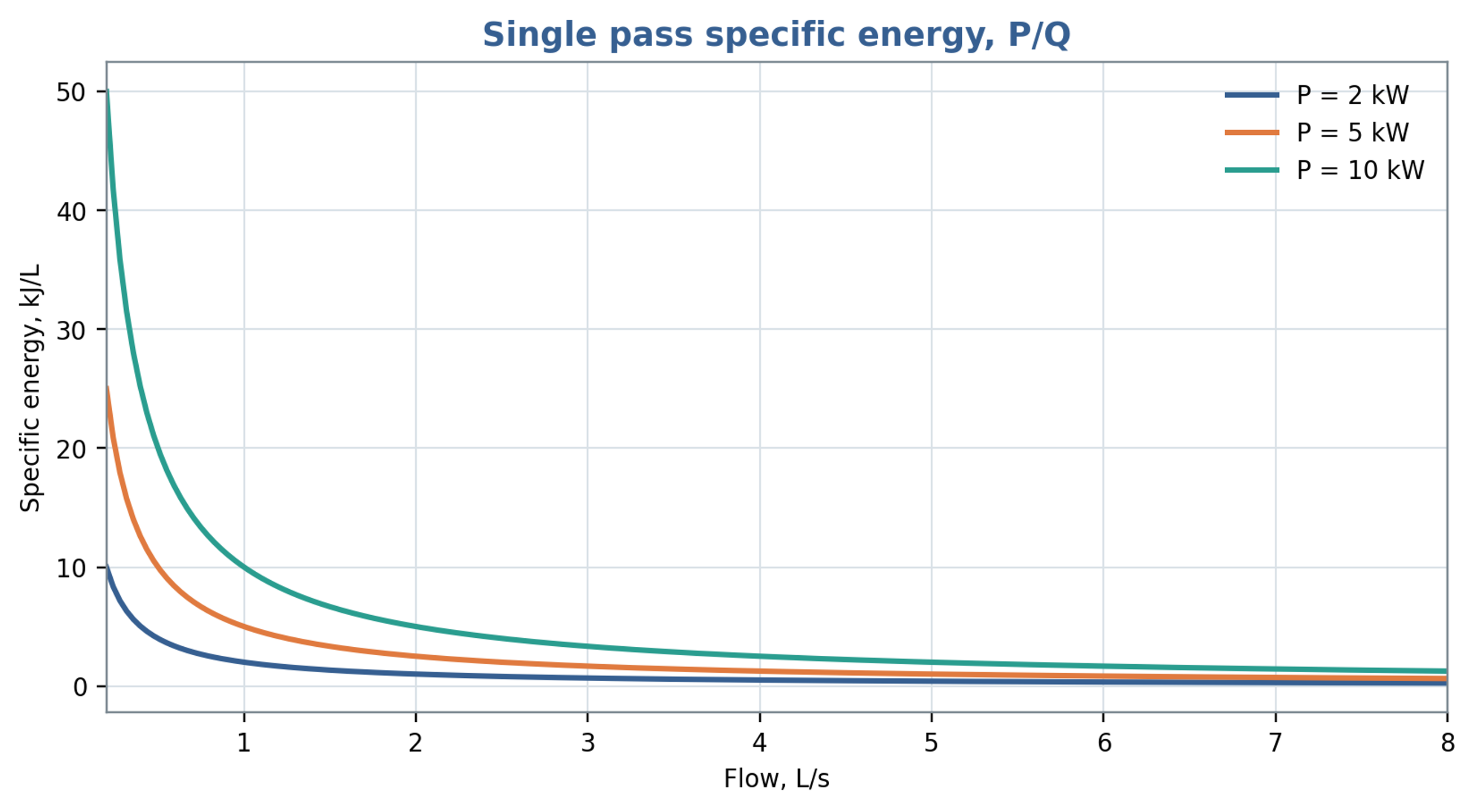
Figure 9.1. Single pass volumetric specific energy as a function of throughput at fixed shaft power, using Equation (9.5). The plotted unit kJ/L is energy per volume; energy per mass additionally requires division by density.

9.4 Heat generation

For a well mixed batch of mass $m$, with approximately constant heat capacity and a fraction ${\eta }_{th}$ of shaft power retained as sensible heat, the temperature rise rate is

For an inline unit, the corresponding temperature rise estimate is $\mathrm{\Delta }T={\eta }_{th}{P}_s/\left(\dot{m}{c}_p\right)$, where the denominator contains mass flow rate and specific heat capacity. The retained thermal fraction depends on the selected boundary and on energy remaining as pressure or motion. Heat removal through the housing, piping, and heat exchanger, as well as heat stored in the equipment, should be included when relevant. Inlet and outlet temperature measurements provide an independent energy balance check when thermal lag, calibration uncertainty, and heat loss are characterized.

For the batch illustrated in Figure 9.2, the retained heating fraction is 0.85 and the assumed constant heat capacity is 4180 J/(kg K). At 30 s, shaft powers of 2, 5 and 10 kW give temperature increases of 0.122, 0.305 and 0.610 °C, respectively. These values establish the seconds time scale of the plotted curves. Over 30 min the corresponding constant property estimates would be 7.32, 18.30 and 36.60 °C; such longer exposure also requires assessment of heat loss and changes in fluid properties.

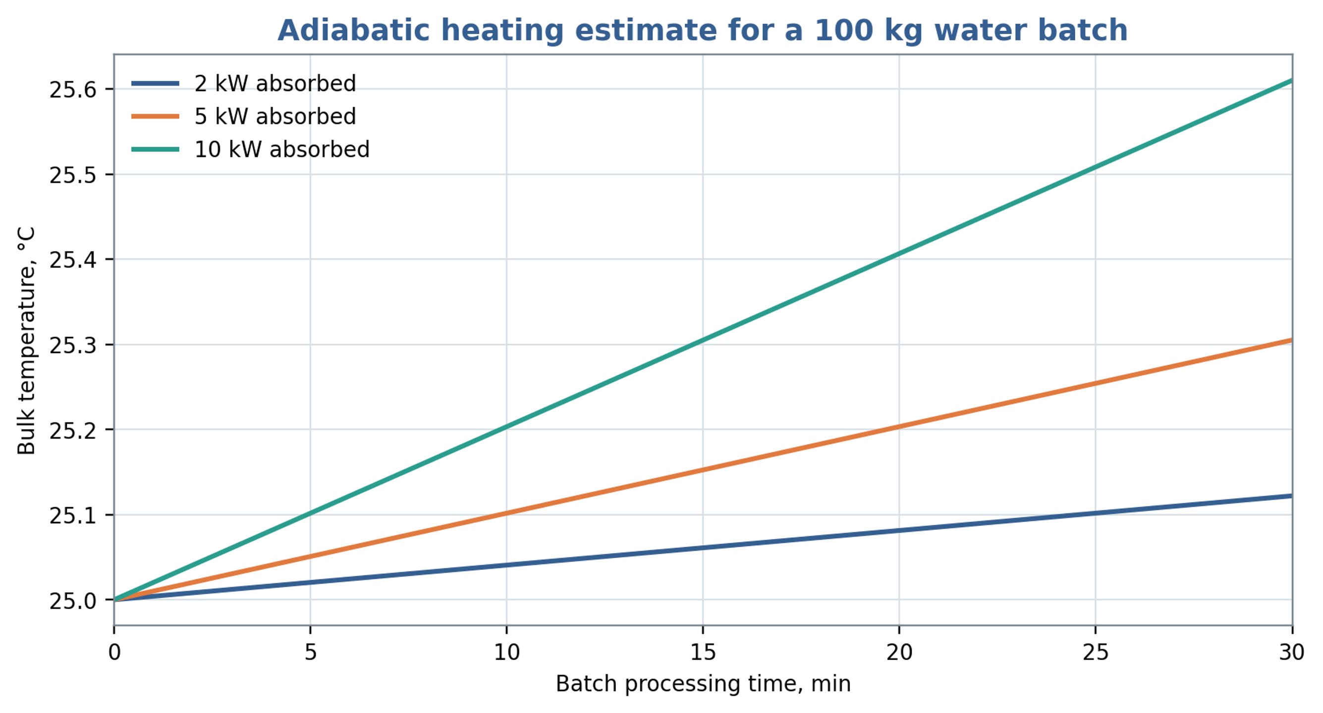
Figure 9.2. Illustrative heating of a 100 kg water batch initially at 25 °C, using Equation (9.7), a heat capacity of 4180 J/(kg K) and ${𝛈}_{𝐭𝐡}=\mathrm{𝟎.𝟖𝟓}$. The plotted time coordinate is in seconds; the embedded min label is incorrect. The legend values are shaft powers before application of the thermal fraction.

9.5 Allocation of power components

A diagnostic allocation of shaft power among hydraulic transport, fluid dissipation, and mechanical loss can be written as

Equation (9.8) provides an accounting structure whose terms must be assigned mutually exclusive physical meanings before they are added. Slot pressure losses already include dissipation caused by jets and turbulence, and cavitation modifies several of those same mechanisms. Adding independently estimated total slot loss, total turbulent dissipation, and total cavitation loss would therefore double count energy. A consistent analysis may allocate losses to separate control volumes or define residual contributions after the directly measured terms are removed. Chervyakov and Yudaev use a related decomposition involving flow kinetic energy, radial and axial gap dissipation, and mechanical loss [1]. Measured shaft power constrains the complete balance.

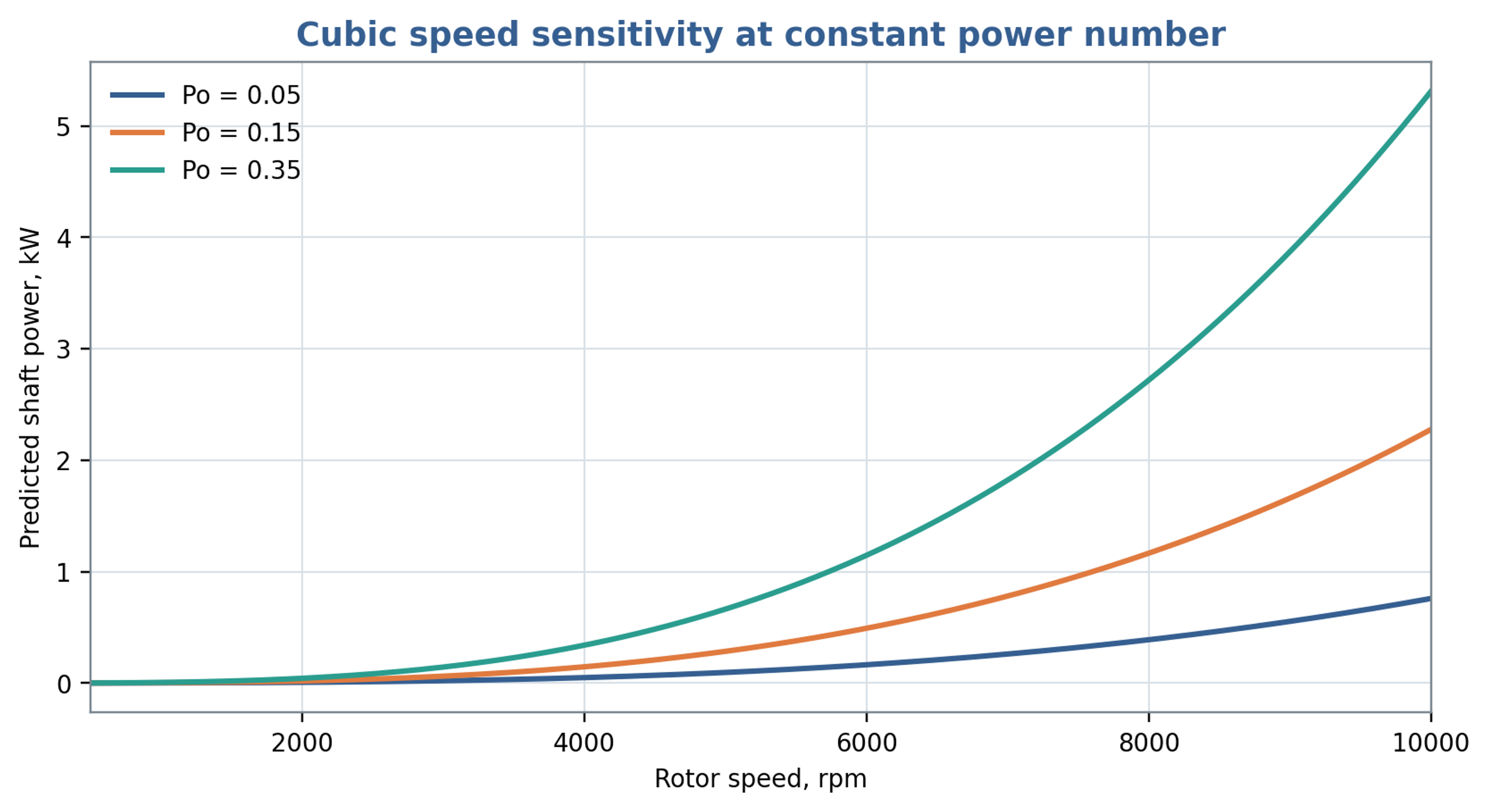
Figure 9.3. Shaft power predicted for selected assumed power numbers using Equation (7.5), $𝐃=\mathrm{𝟖𝟎}$ mm and a density of 1000 kg/m³. These curves illustrate sensitivity to the coefficient and are not validated power predictions for the worked example.

Table 9.1. Power measurements and deductions

Measurement	Directly obtained	Derived quantity	Common error
Shaft torque and speed	$P_s=T\omega$	Fluid load after no load subtraction	Using motor nameplate power as actual shaft power
Inlet and outlet absolute pressure	$\mathrm{\Delta }p$ and cavitation margin	$Q\mathrm{\Delta }p$, $\sigma$	Using only gauge pressure near vacuum
Flow rate	$Q$ or $\dot{m}$	$P/Q$, residence time, flow coefficient	Ignoring pulsation or calibration fluid
Temperature rise	Sensible heat	Approximate thermal fraction	Ignoring heat loss and sensor lag
Fast pressure and flow	$p^{\prime }(t)$ and $q^{\prime }(t)$	$\overline{p^{\prime }{q}^{\prime }}$, spectra, phase	Unsynchronized sampling or inadequate bandwidth
Electrical input	Drive consumption	Shaft power after efficiency correction	Treating variable frequency drive display as torque calibration

9.6 Experimental determination of power characteristics

Experimental power correlations require a defined measurement boundary. James et al. corrected measured torque for bearing losses and instrument offsets before determining power constants for several batch mixer sizes. Their results distinguish laminar, transitional and fully turbulent operation and show that the constants can depend on both mixer scale and workhead geometry. In particular, changes in flow area and removal of the stator screen altered the power characteristics. Consequently, a coefficient determined for one head should be used with its stated Reynolds number definition, rheological conditions and geometric limits. The reported turbulent torque dependence on rotational speed squared also provides a consistency check when cubic power scaling is assumed [25].