Design and Operating Principles of Rotor-Stator Mixers

9. Theoretical Basis of Hydromechanical Processes in Rotor-Stator Systems

Theoretical analysis of rotor-stator mixers examines the kinematic and dynamic flow parameters governing dispersion, homogenization, and mass transfer. A key determinant of mechanical action is rotor tip speed $U_t$, which combines working element geometry, particularly rotor diameter ($D$) with drive kinematics, including rotational frequency ($n$) and angular velocity ($\omega$).

The analytical relationship between rotor diameter, rotational speed, and tip speed given in Equation (2.2) provides an estimate of the potential shear deformation and energy transfer to the flow [1].

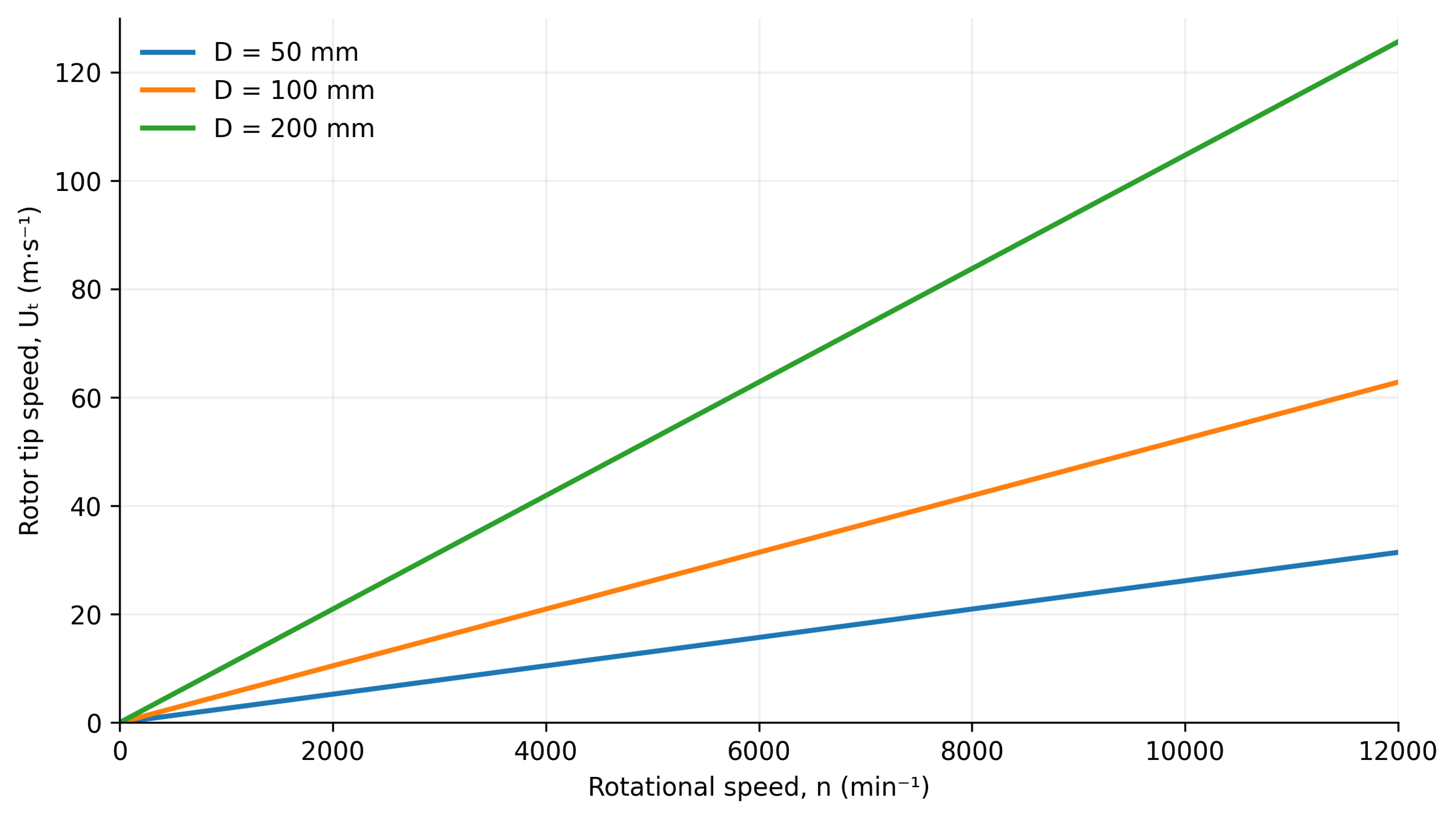
Figure 9.1. Calculated rotor tip speed as a function of diameter and rotational speed according to Equation (2.2) [1].

9.1 Velocity Gradients and Intensive Shear Stresses

In first approximation, the relative fluid velocity changes across an effective gap of width g. The nominal shear rate is

where γ̇ₙₒₘ is the nominal shear rate, Uᵣₑₗ is relative velocity in the gap, and g is the effective gap width.

For a Newtonian continuous phase, viscous shear stress is related to shear rate by

where τ is shear stress and μ is dynamic viscosity.

The estimate based on the gap is useful for comparison but does not fully describe local velocity fields. Leakage, recirculation, blade wakes, and acceleration through stator openings can produce local deformation rates both above and below the nominal estimate. In Rueger's laminar batch experiments, droplet breakup corresponded to simple shear rates roughly twice those estimated from the nominal gap. That factor is specific to the tested configuration and is not a universal correction [2].

For a non-Newtonian formulation, the preceding stress equation represents only the Newtonian limiting case. Predictions additionally require an appropriate constitutive model and, when relevant, allowance for yield stress, thixotropy, or elasticity. Viscosity measured at a single low shear rate cannot be used to represent the entire high-gradient working region.

Fluid accelerating through a converging passage also undergoes extension. A representative axial extensional strain rate is

where ε̇ₓ is the axial extensional strain rate and uₓ is the velocity component in the x direction.

During extension, a fluid element elongates in one direction and contracts in others. This mechanism is important for deformable interfaces and polymeric materials, although the outcome depends on the deformation history and material response. Leading blade edges, wedge surfaces, and entrances to openings generally produce mixed flows rather than the uniform shear of an ideal rheometer.

The ratio of inertial to viscous effects on the rotor scale is defined as

where Reᵣ is the rotor Reynolds number, ρ is density, N is revolutions per second, D is rotor diameter, μ is dynamic viscosity, and ν is kinematic viscosity.

An additional Reynolds number is defined using the clearance and its associated relative velocity:

where the characteristic scales for Re₉ are relative velocity Uᵣₑₗ and gap width g.

The rotor and gap Reynolds numbers describe different scales. A high value at the rotor scale can coexist with relatively ordered flow within a narrow viscous gap. Conversely, separation at an opening may generate fluctuations that a simple gap model does not represent. Neither definition establishes a universal transition threshold for all mixer geometries.

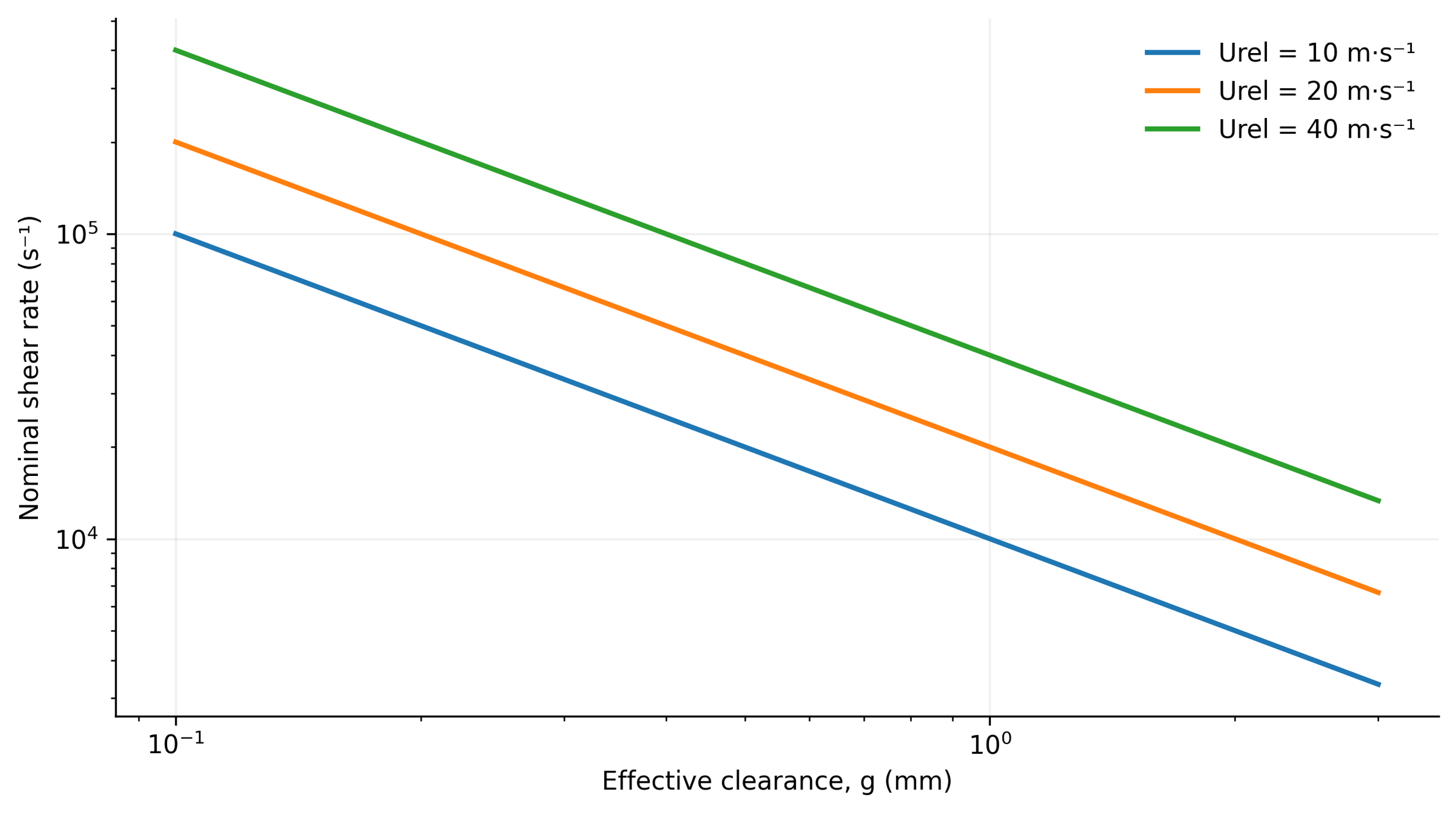
Figure 9.2. Nominal gap shear rate for three relative velocities calculated using Equation (9.1). Effective clearance is a model input and does not account for local gradients near openings or in wakes [1].

9.2 Torque, Power, Pumping, and Energy Dissipation

Torque T and rotational frequency determine the mechanical power transmitted by the shaft:

where Pₛ is shaft power, N is rotational frequency in s⁻¹, and T is torque.

Shaft power is not equal to the power dissipated within the liquid. Mechanical losses and net hydraulic power transferred to the flow must be considered before calculating dissipation. Loss characteristics approved by the manufacturer may be compared with calorimetry and flow and pressure measurements. Mechanical seals must not be operated dry merely to establish a baseline loss measurement. Nearly all dissipated energy ultimately becomes heat, but calorimetric analysis must account for heat transfer and energy crossing the boundaries of the control volume.

The power number is defined using power dissipated in the liquid:

where Po is the power number and $P_{diss}$ is power dissipated in the processed liquid.

Dimensionless throughput and pressure rise are expressed as

where Φ is the flow coefficient and Q is volumetric flow rate.

where Ψ is the pressure coefficient and Δp is the pressure change across the mixer, positive for pressure generation and negative for pressure consumption under the specified sign convention.

For a positive useful pressure rise, the hydraulic power fraction is

where ηₕ is hydraulic efficiency. A low value of ηₕ is not necessarily a disadvantage for a mixer because intentional viscous dissipation is often the primary process objective.

Rueger found that the dissipative power component of an IKA inline mixer was nearly independent of flow rate over part of the tested turbulent range. The measurements were described by a correlation involving effective diameter and stage count [2]. Computational analyses of a Silverson inline head demonstrate the importance of unsteady rotor-stator interactions and turbulence model selection for predicted throughput and power [3]. These findings support calibration for each geometry rather than adoption of a single power number for all high shear mixers.

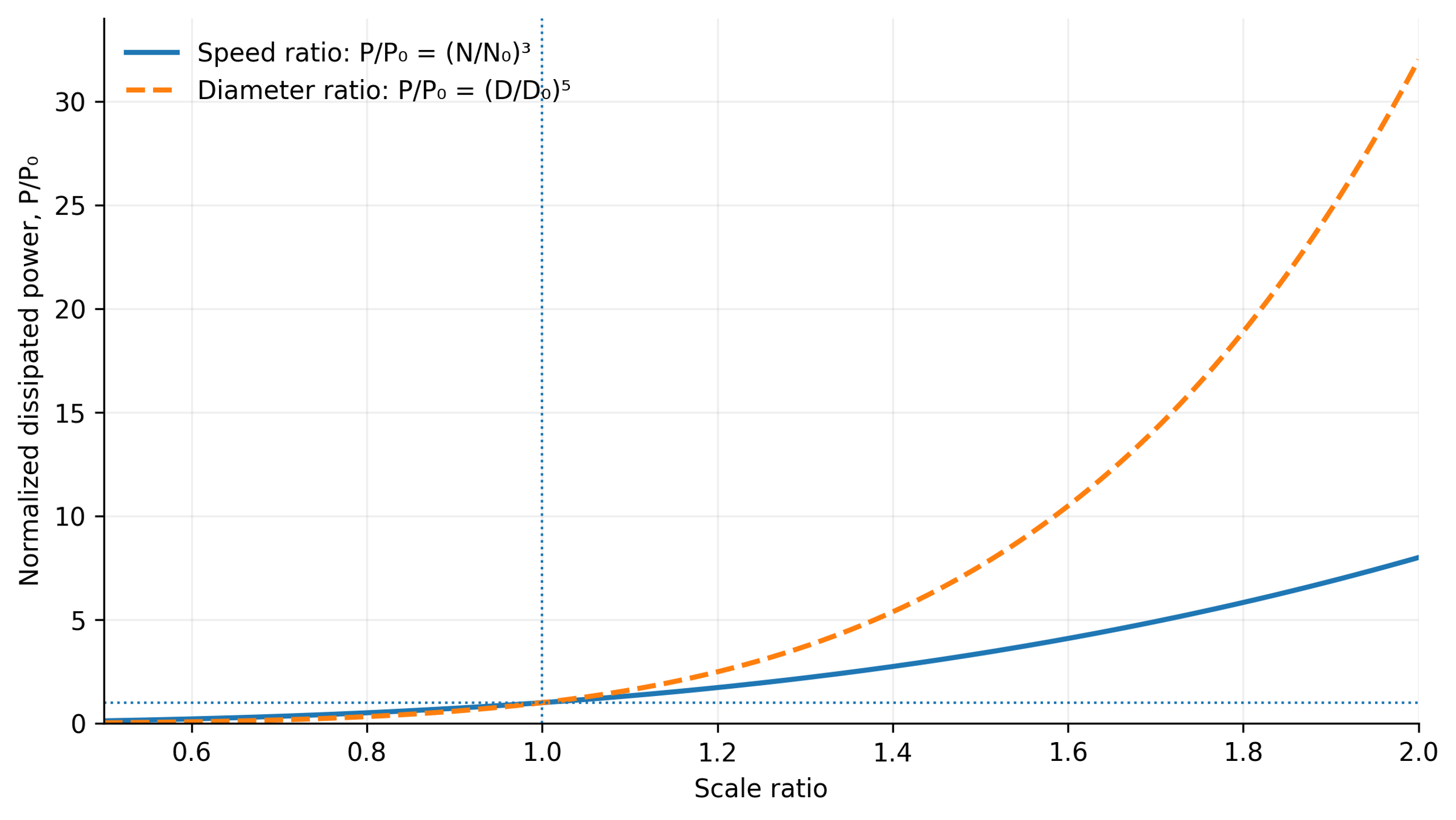
Figure 9.3. Idealized sensitivity of power to rotational speed and rotor diameter based on Equation (9.7), assuming constant density and power number. Only the indicated independent parameter varies on each curve [1].

The definition of the power number must be stated whenever results are compared. Equation (9.7) uses dissipated power, whereas experiments may report measured shaft power. The values agree only if the neglected terms are genuinely small. A negative pressure rise denotes a mode that consumes pressure head; in that case, Equation (9.10) is a signed power ratio rather than the conventional positive efficiency of a pump.

The mean rate of energy dissipation per unit fluid mass in a specified averaging volume V is

where $ϵ$ is the mean specific dissipation rate in W/kg; $P_{diss}$ is dissipated power; ρ is density; V is the averaging volume.

For a selected active region, volumetric dissipation is estimated by dividing the power dissipated there by the region volume:

where εᵥ,ₗₒ꜀ is the local volumetric energy dissipation rate in W/m³, Pₗₒ꜀ is the power dissipated in the active region, and Vₐ is its volume.

Dissipation Rate Is Not the Same as Accumulated Energy Density

Energy dissipation rate is expressed as power per unit mass or volume, for example W/kg or W/m³. Accumulated specific energy is expressed in J/kg or J/m³ and incorporates treatment duration or flow rate. These metrics address different questions: local dissipation characterizes instantaneous deformation, while accumulated energy describes the dose delivered per pass or per batch.

In steady inline operation, the dissipated energy per unit volume of processed material is

where Eᵥ,ꜰᴛ is inline specific volumetric energy in J/m³, a quantity dimensionally equivalent to pressure in Pa.

For a batch operated at constant dissipated power over a duration t, the nominal accumulated energy dose is

where Eᵥ,ʙ is the nominal batch specific volumetric energy and Vₜ is the batch volume.

If heat exchange, phase changes, and changes in specific heat are neglected, the corresponding temperature increase is

where ΔT is the temperature rise, m is the processed mass, cₚ is specific heat capacity, and Eₘ is accumulated energy per unit mass.

Temperature rise is an essential process constraint. An accumulated energy dose of 100 kJ/kg in a fluid with specific heat capacity 4.18 kJ/(kg·K) gives an adiabatic increase of approximately 24 K. Temperature affects viscosity, interfacial tension, vapor pressure, and reaction rates. Consequently, the hydrodynamic regime and the material response may change even at constant shaft speed.

For inline operation, the mass used in the thermal relation is the quantity processed during the corresponding interval. In a batch process, it is the mass of the batch. If viscosity, torque, or cooling changes during treatment, the constant-power approximation should be replaced by a time-dependent energy balance. Temperature history should be reported together with energy dose rather than treated as a secondary operating parameter.

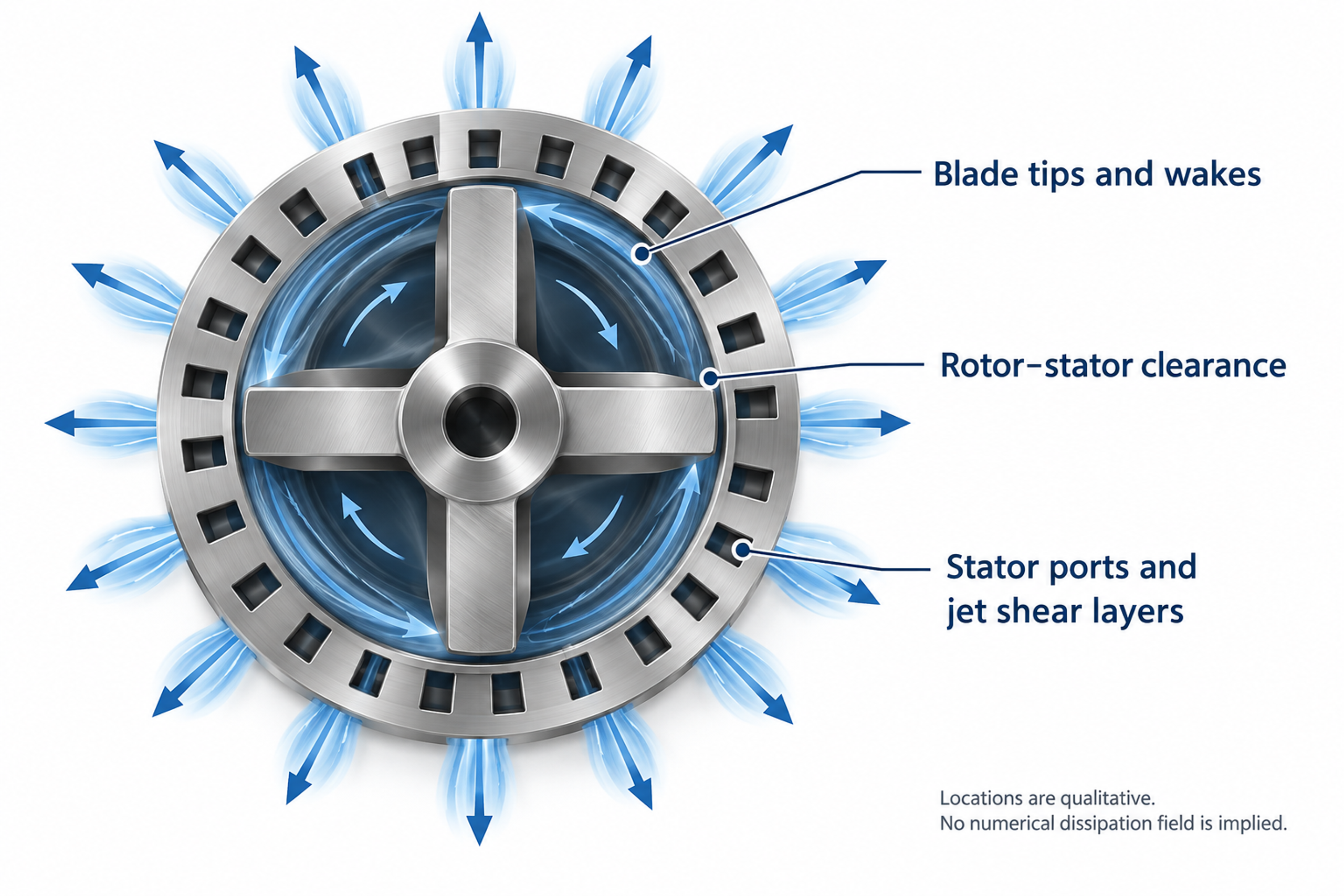
Figure 9.4. Qualitative diagram of regions of intense deformation and dissipation at blade tips, within the gap, and in stator jets. [1, 2, 3].

9.3 Mechanisms of Particle and Droplet Breakup in Rotor-Stator Mixers

Hydrodynamic loading must overcome either interparticle cohesive forces or capillary resistance to break agglomerates or deform droplets. Depending on structural strength and treatment intensity, breakup may occur through gradual surface erosion of agglomerates or rapid fragmentation into many smaller pieces. Bałdyga and Malik compare deagglomeration equipment using local energy dissipation and specific energy demand while considering the different mechanisms of stress generation. In rotor-stator machines operating without cavitation, breakup primarily results from hydrodynamic deformation, including shear and extension, which should not be confused with impact grinding in bead mills or abrasion of primary crystals [17].

U.S. Patent 6,000,840 provides illustrative empirical comparisons: median particle diameters of 9.7, 3.2, and 2.0 μm were reported for a high speed disperser, a conventional rotor-stator unit, and a specialized wedge rotor, respectively, while corresponding specific surface areas were 2.2, 3.3, and 5.2 m²/g. The patent also records changes in formulation and equipment settings between tests. These measurements therefore describe particular experimental runs, not a controlled isolation of rotor geometry at identical composition and specific energy input and cannot establish a universal ranking of equipment efficiency [9].

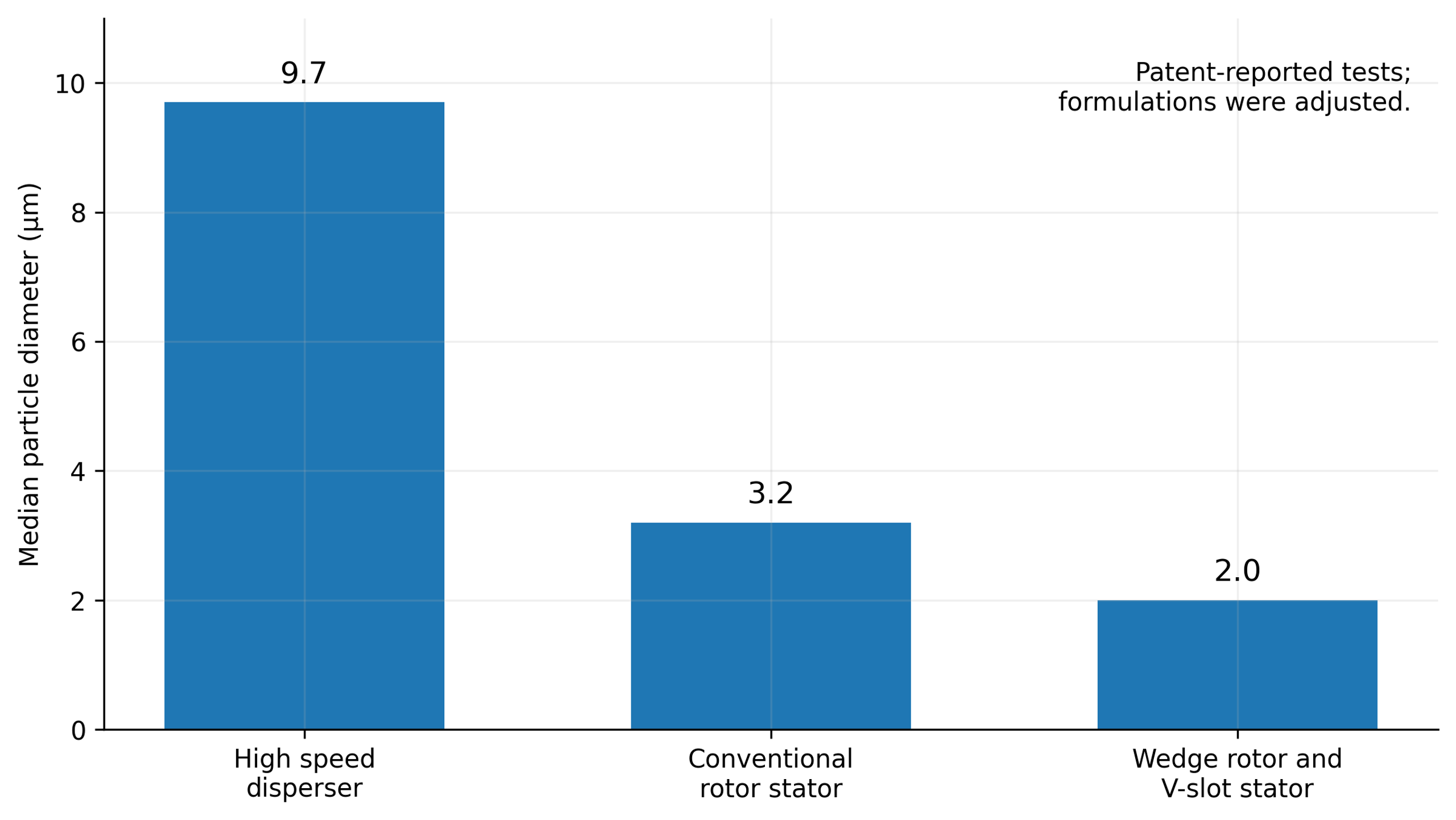
Figure 9.5. Median particle diameters reported in U.S. Patent 6,000,840. Corresponding specific surface areas were 2.2, 3.3, and 5.2 m²/g. Changes in composition and operating settings prevent interpretation as a universally controlled performance ranking [9].

The deagglomeration literature relates stronger processing to changes in the resulting agglomerate size distribution [17]. A separate calculation based on Equation (9.32) illustrates liquid droplet breakup and the sensitivity of inertial-range scaling to dissipation and interfacial tension. These curves are not Aerosil measurements, and a liquid droplet model cannot be applied directly to the cohesive strength of solid agglomerates.

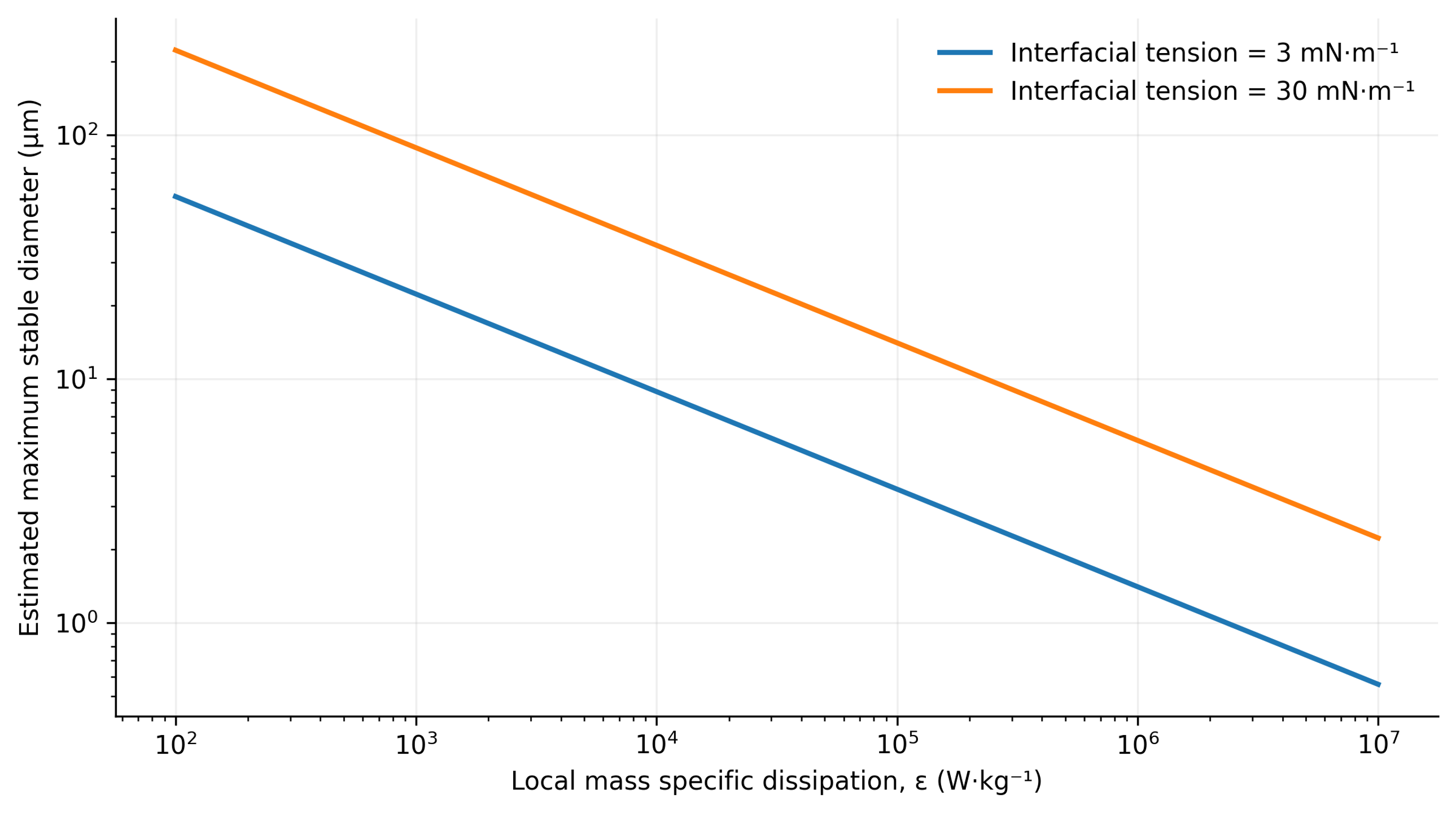
Figure 9.6. Calculated inertial-range scaling of maximum stable droplet diameter using Equation (9.32), with density 1000 kg/m³ and an illustrative coefficient Cₕ = 0.725 [1].

9.4 Hydrodynamic Cavitation in Rotor-Stator Mixers

Hydrodynamic cavitation involves nucleation and rapid growth of cavities containing vapor or gas in localized low-pressure regions, for example behind rotor blades, within rotor-stator gaps, or at the entrances to calibrated stator openings. Subsequent transport into higher pressure regions produces rapid condensation or collapse. Cavitation bubble collapse can generate strong pressure waves, high speed microjets, and extreme localized temperatures and pressures that may erode metallic working surfaces.

Dissolved gas and gas filled nuclei substantially influence cavitation dynamics, but expansion of a gas bubble is not necessarily equivalent to collapse of a vapor cavity. Under suitable conditions, controlled cavitation can intensify dispersion, homogenization, and interfacial mass transfer through highly localized energy release. Uncontrolled cavitation, however, can degrade hydraulic performance and cause unacceptable vibration, noise, and premature equipment wear. Analysis of pressure history of the flow and the location of bubble collapse is therefore more informative for process performance and safety than simply observing bubbles in the medium [18, 19, 20].

A simplified steady relation for mechanical energy can be used to compare two channel sections:

where p₁ and p₂ are static pressures, U₁ and U₂ are mean velocities, and Δpₗ represents irreversible pressure losses, including elevation effects when necessary.

This relation shows conversion between static pressure and kinetic energy in a channel but does not represent the complete energy balance of an operating rotor, which also involves shaft work, centrifugal effects, unsteadiness, and three-dimensional flow. A common dimensionless indicator of pressure margin is the cavitation number,

where σ꜀ is the cavitation number, pᵣₑꜰ is a reference absolute pressure, pᵥ is vapor pressure, and Uᵣₑꜰ is the chosen local reference velocity.

A lower value indicates less pressure margin relative to the selected velocity scale, not a universal cavitation threshold. The absolute reference pressure, temperature, vapor pressure, and velocity reference location must be reported. Nuclei concentration, dissolved gas, and surface condition can shift the onset even under nominally identical operating settings. Cavitation numbers should therefore be supplemented with local pressure measurements, validated simulations, or direct observation.

The radial motion of a spherical cavity in an incompressible liquid is described by the Rayleigh-Plesset equation:

where R is bubble radius; $p_B$ is pressure inside the bubble; p∞ is the far field liquid pressure; σ is surface tension; and dots denote differentiation with respect to time [18, 19, 20].

Using the Rayleigh-Plesset equation requires a model for internal bubble pressure and a specified or coupled calculation of the external pressure history. The equation alone does not predict nuclei concentration, asymmetric microjet formation, or interactions between neighboring bubbles. Its incompressible form is also insufficient to describe the final, strongly compressible phase of collapse in detail. These limitations are particularly significant when extrapolating a single bubble model to cavitation mixer performance [20].

For an initially stationary empty cavity collapsing under a constant positive pressure difference, Rayleigh's estimate of collapse time is

where t꜀ is collapse time and R₀ is the initial cavity radius [18].

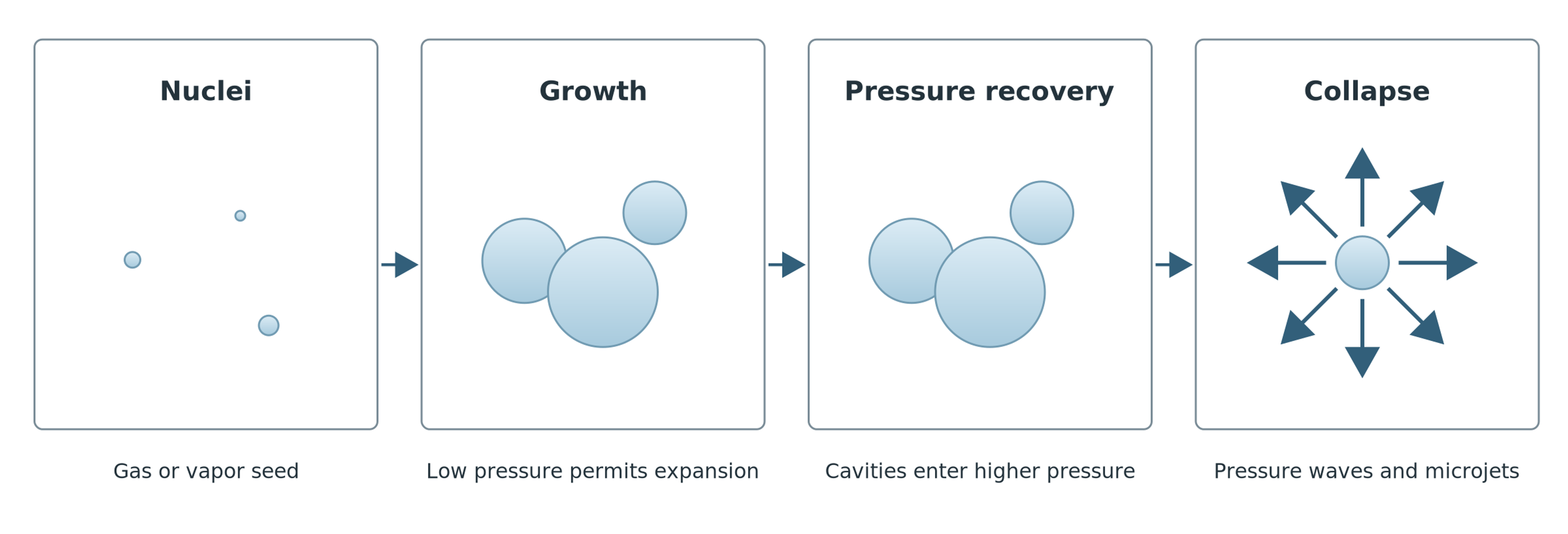
Figure 9.7. Cavity growth, transport to a region of pressure recovery, and collapse. [1].

Whereas an ordinary mixing head under sufficiently high static pressure can operate without cavitation even at high tip speeds, dedicated rotational cavitation reactors are designed specifically to create pronounced low pressure regions. Their working elements may incorporate profiled holes, grooves, pins, or features that promote flow separation that intensify local pressure variations. Zhang and colleagues demonstrated that hole geometry substantially affects vapor distribution, vortex structure, and pressure fluctuation amplitude in such reactors [21]. Their results establish sensitivity to the particular flow geometry examined but cannot be generalized into a universal cavitation law for all rotor-stator mixers.

Analytical and numerical estimates of cavity collapse dynamics often assume that a cavity starts from rest and experiences a constant positive driving pressure difference. In actual process fluids, collapse is strongly modified by factors including:

• The presence of noncondensable gas in nuclei.

• Fluid rheology and viscosity.

• Interfacial surface tension.

• The finite speed of sound in a two phase flow.

• Proximity to solid boundaries such as chamber walls and rotor-stator surfaces.

Consequently, a calculated theoretical cavity-collapse time should not be presented as an experimentally measured event duration or used as a reliable quantitative predictor of erosive damage to structural materials [18, 19, 20, 21].

9.5 Acoustic Oscillations and Hydrodynamic Pressure Pulsations

Periodic interaction between moving rotor elements and stationary stator passages generates regular pressure oscillations even in a single phase incompressible liquid. Successive rotor teeth, blades, or holes pass stationary features at a characteristic element passage frequency, while nonlinear partial obstruction of the passages produces higher harmonics in the pressure spectrum.

Rotor-pulsation apparatuses deliberately exploit this flow modulation using toothed crowns, profiled channels, and concentric working rings to intensify mixing and dispersion [4, 5, 6, 7]. In spectral analysis, the resulting discrete tonal pressure signal must be distinguished from broadband high-frequency turbulence and the short pressure impulses produced by localized collapse of cavities containing vapor or gas.

Periodic rotor-stator interactions produce pressure oscillations even in single phase liquids. Repeating rotor features pass stationary openings at a characteristic frequency, while partial obstruction generates higher harmonics. Rotor-pulsation designs use teeth, channels, and working rings to create this modulation [4, 5, 6, 7]. The resulting signal must be distinguished from broadband turbulence and the impulsive components of bubble collapse.

A periodic pressure signal can be represented as the sum of a mean component and harmonics:

where p̄ is mean pressure, Aₖ is the amplitude of harmonic k, k is the harmonic index, and φₖ is its phase.

For the restricted case of a propagating plane acoustic wave, the mean sound intensity is estimated by

where I is sound intensity, pᵣₘₛ is root-mean-square acoustic pressure, ρ is density, and c is sound speed.

The plane wave expression is valid only under specific conditions. Pressure measured near a mixing head includes hydrodynamic fluctuations, reflections, and coupling to structural vibration; its total rms value cannot automatically be treated as the pressure of a propagating plane wave. The Strouhal number provides a separate measure comparing an observed frequency with a convective time scale:

where St is Strouhal number, f is frequency, L is a characteristic length, and U is a characteristic velocity.

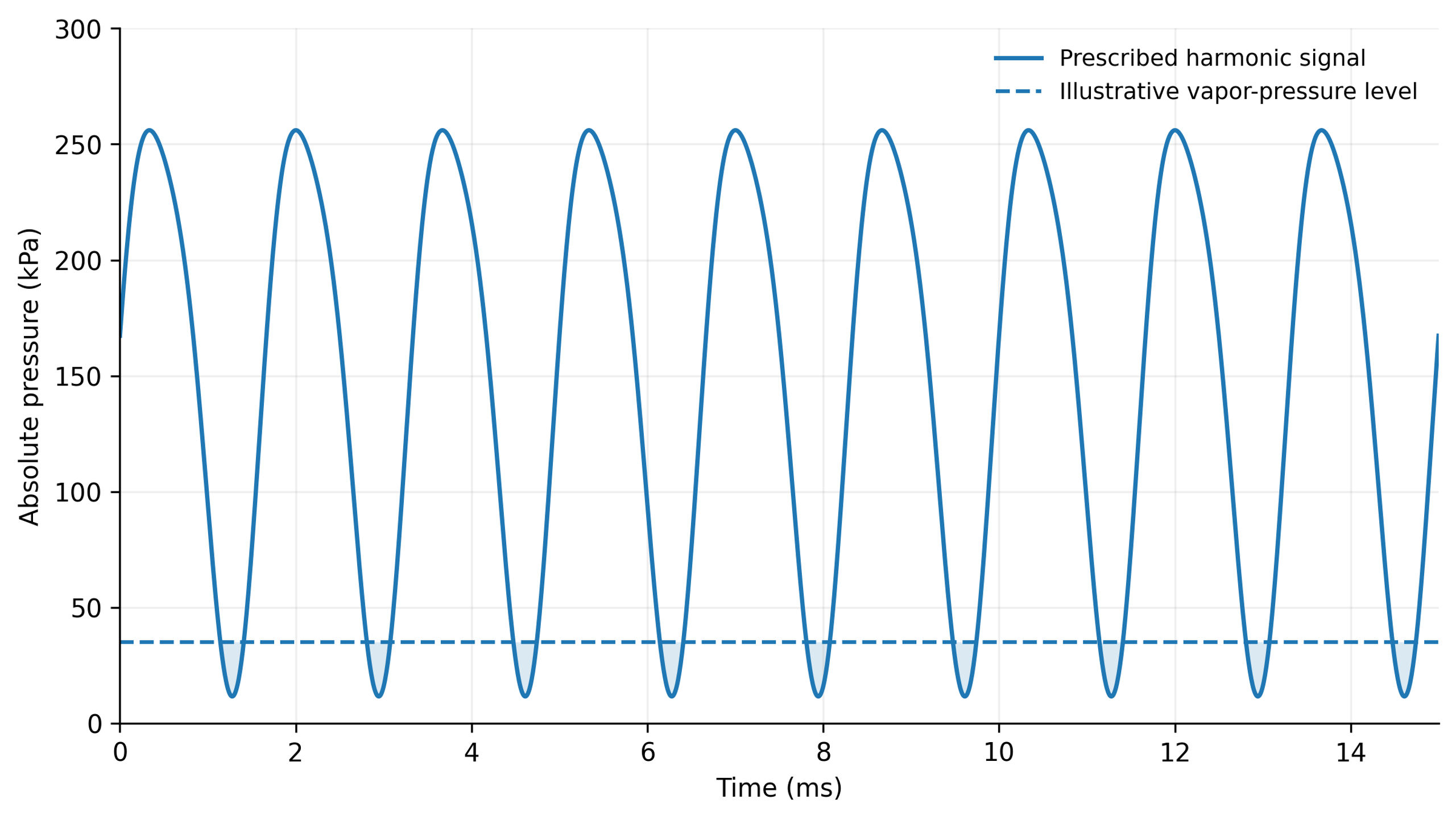
Figure 9.8. Illustrative harmonic pressure signal based on Equation (9.20): mean pressure 150 kPa, fundamental amplitude 120 kPa at 600 Hz, and a 20 kPa second harmonic with phase π/3. The 35 kPa reference level is illustrative; intervals below that level do not represent a calculated two-phase flow [1].

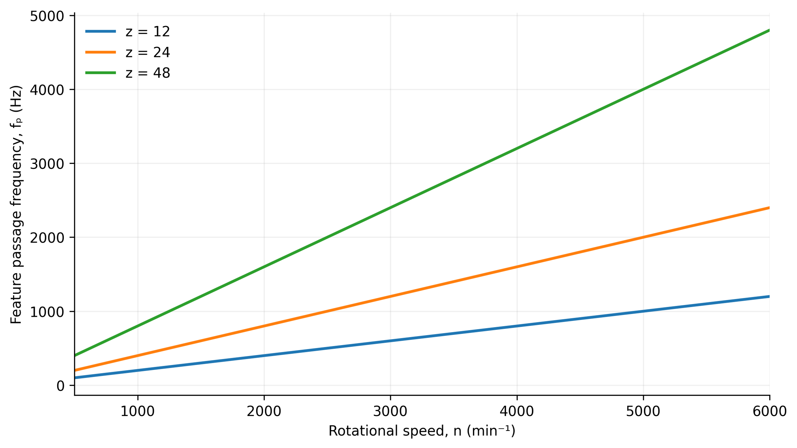
Figure 9.9. Calculated passage frequencies for 12, 24, and 48 repeating elements using Equation (2.3). The relation does not determine amplitude or additional spectral components [1].

A spectral maximum at the element passage frequency and its harmonics helps identify direct rotor forcing. Sidebands and broadband components must be interpreted in conjunction with operating conditions and the measurement system. In a rotational cavitation reactor studied by Zhang and colleagues, 24 circumferential openings produced a dominant frequency component equal to 24 times the shaft rotation frequency. Hole diameter influenced pressure amplitude in that specific geometry [21].

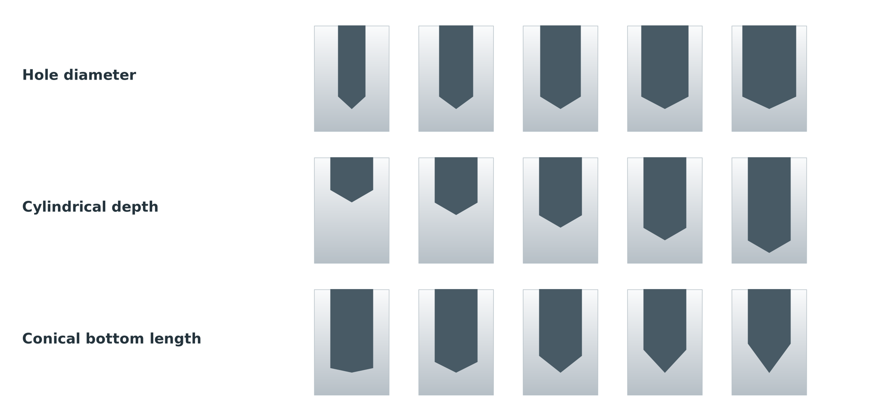
Figure 9.10. Families of hole geometries varying in diameter, cylindrical depth, and conical bottom length [21].

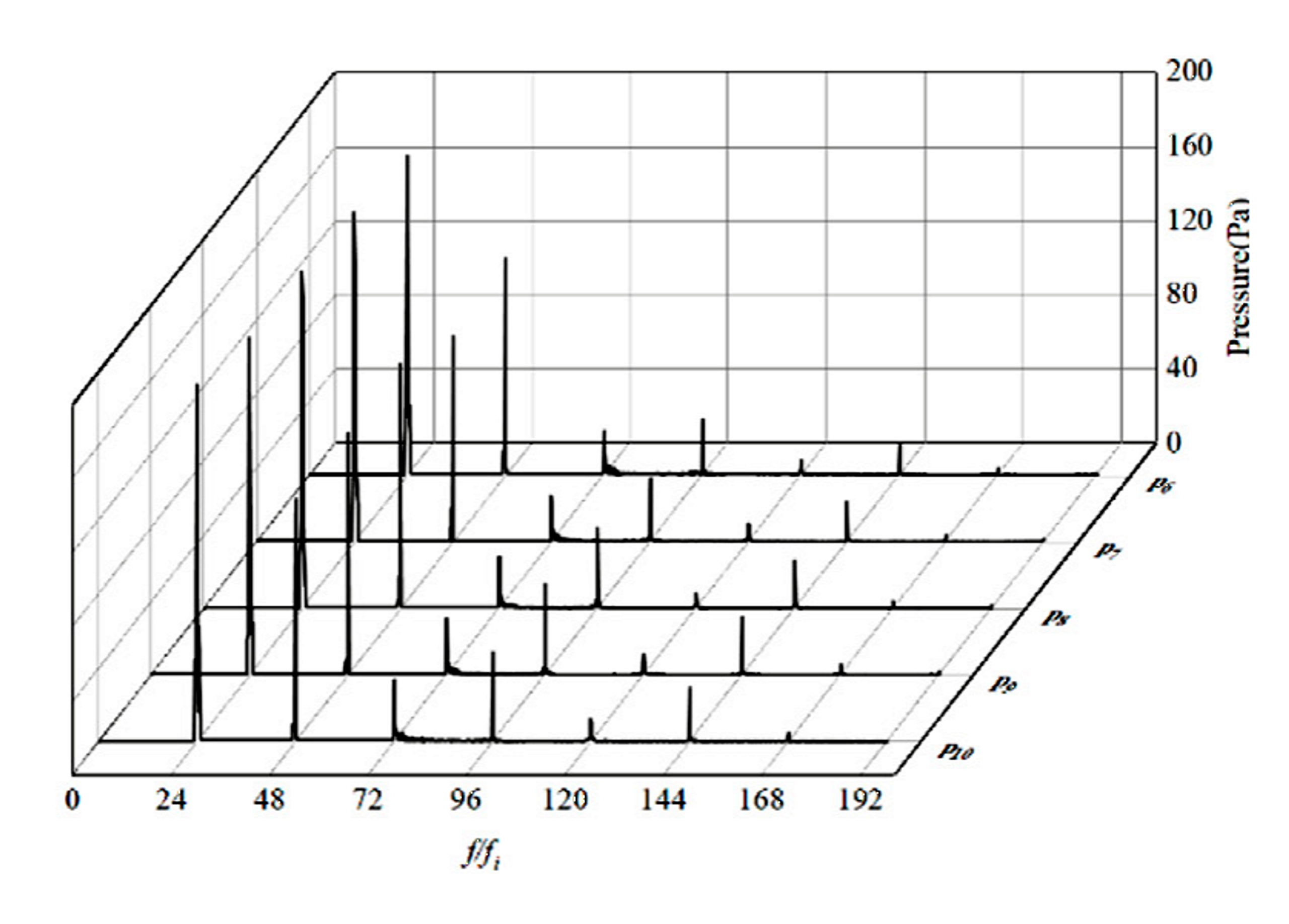
Figure 9.11. Published pressure spectra for the largest hole diameter, 19 mm, at five measurement locations. Reproduced under CC BY 4.0 [21].

The spectra in Figure 9.11 are a selected excerpt from a published study, not newly digitized experimental data. The original axes and curves are retained. The idealized harmonic wave shown elsewhere in this section illustrates a signal representation and is not a numerical simulation of two-phase cavitation.

9.6 Spatial and Temporal Scales of Turbulence and the Fine Structure of Dissipation

In strongly inertial flows, separation at rotor blade edges and high-velocity jets leaving stator openings produce fluctuations over a broad range of spatial and temporal scales. Energy dissipation is markedly nonuniform and intermittent within rotor-stator mixers. Integral measures averaged over the tank therefore cannot represent the extreme local mechanical loading in the narrowest gaps or at stator exits. In Rueger's tested inline geometry, the peak local dissipation rate was approximately nine times the average over the mixer. That observation concerns a particular design and cannot be extrapolated as a universal correction factor [2, 3].

Kolmogorov microscales are used to describe the small scale structure of turbulence and local micromixing in high shear regions. The Kolmogorov length scale ($\eta$) characterizes the smallest eddies where kinetic energy is dissipated viscously and is defined by

where η is Kolmogorov length scale, ν is kinematic viscosity, and ε is local specific energy dissipation rate.

where τᵨ is Kolmogorov time scale.

where uᵨ is Kolmogorov velocity scale [22].

For a passive scalar in the viscous-convective regime at high Schmidt number, the Batchelor scale is

where ${\eta }_B$ is the smallest scalar diffusion scale and Sc is the ratio of kinematic viscosity to molecular diffusivity [23].

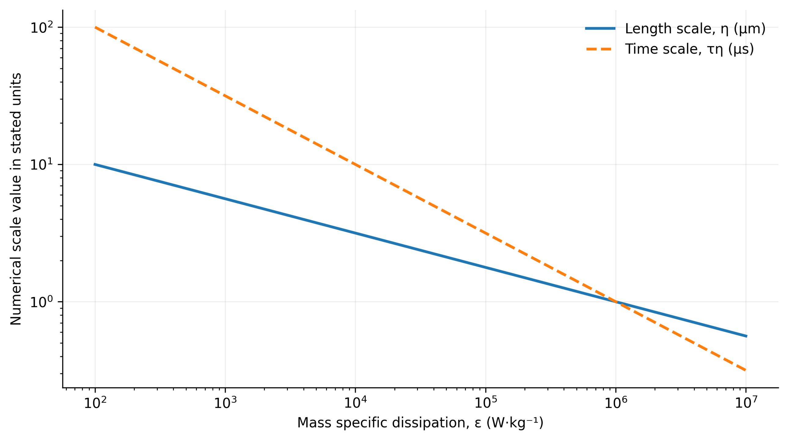
Figure 9.12. Calculated Kolmogorov length and time scales at kinematic viscosity 1.0 × 10⁻⁶ m²/s, using Equations (9.23) and (9.24) [1].

Although fundamental, the Kolmogorov and Batchelor scales describe idealized local turbulence and passive scalar diffusion. They cannot be equated directly with the minimum achievable droplet or solid particle diameter in real dispersions. Use of these scales requires validation of flow assumptions and explicit local dissipation averaging. The Batchelor relation is not a universal mixing length at small Schmidt numbers ($Sc\ll 1$), or in polydisperse materials with complex rheology such as viscoelasticity or yield stress.

For a droplet or solid particle of diameter ($d$) lying in the inertial subrange of developed turbulence, dynamic stress induced by velocity fluctuations at eddies of comparable size can be estimated from Kolmogorov-Obukhov scaling:

For a particle or droplet in the inertial subrange, stress at the eddy scale is approximated by

where τᵢ is the inertial stress at scale d and Cᵢ is a coefficient of order unity.

For an object smaller than the Kolmogorov length, viscous stress at the smallest turbulent scale can be estimated by

where τᵥ is viscous microscale stress and Cᵥ is a coefficient dependent on the stress definition.

These relationships provide a basis for balancing disruptive hydrodynamic forces against capillary and viscous restoring forces in models of emulsification and deagglomeration.

9.7 Droplet Breakup, Interfacial Area, and Micromixing

In emulsification and dispersion processes, the breakup of liquid droplets, formation of interfacial area, and micromixing depend on the balance between externally applied hydrodynamic deformation and internal capillary restoring forces.

For a droplet in developed inertial turbulence, the primary dimensionless criterion comparing disruptive fluctuating stresses with interfacial tension is the droplet Weber number:

where Weᵈ is droplet Weber number, d is droplet diameter, and σᵢ is interfacial tension.

For viscous shear, the corresponding parameter is the capillary number,

where Ca is capillary number and μ is continuous-phase viscosity.

The Ohnesorge number describes the influence of dispersed-phase viscosity:

where Oh is Ohnesorge number, and μᵈ and ρᵈ are dispersed-phase viscosity and density.

Equating turbulent inertial loading with capillary restoring forces yields a scaling relation for the maximum stable droplet diameter:

where dₘₐₓ is the maximum stable droplet diameter and Cₕ is an empirical coefficient. The expression is a scaling relation, not a universal calibration of mixer performance.

This relation describes an illustrative scaling behavior of emulsification rather than a universally calibrated mixer model. The empirical coefficient $C_H$ and the critical breakup conditions depend on the mathematical definitions, data analysis methods, and rheological properties of the phases. The relation is most appropriate for droplets within the inertial subrange, provided that dispersed-phase viscosity, confinement, and recoalescence do not dominate.

In practice, maximum stable droplet diameter ($d_{\max }$) must not be equated with Sauter mean diameter ($d_{32}$) without a statistical model for droplet size distribution. If creation and stabilization of fresh interfaces occur on the time scale of hydrodynamic exposure, dynamic rather than equilibrium interfacial tension becomes important.

The Sauter mean diameter relates dispersed-phase volume to interfacial area through the number distribution:

where nᵢ is the number of droplets in size class i and dᵢ is the diameter of that class.

For spherical droplets with dispersed-phase volume fraction φᵈ, the interfacial area per unit mixture volume is

Where a is the specific interfacial area per unit mixture volume.

The same area relationship applies to a polydisperse set of spherical droplets if d₃₂ is calculated from the moments of the number distribution. This follows directly from summing the surface areas and volumes of spheres. No sphericity, inaccessible surfaces, and uncertainty in the dispersed phase volume fraction require separate consideration; a single diameter measurement does not determine the actual accessible interfacial area.

A common estimate of micromixing time uses the smallest turbulent time scale:

where tᵨ is micromixing time and Cᵨ is a model coefficient.

The relationships link local deformation, interfacial properties, and exposure time with the expected processing outcome. They do not, however, close the model for an evolving size distribution. Breakup competes with coalescence, adsorption, and transport, while rheological changes alter the flow itself. Once a useful limiting state is approached, further processing mainly increases heating and wear. The preferred operating target is therefore the minimum reproducible energy dose meeting product requirements, not maximum treatment duration.

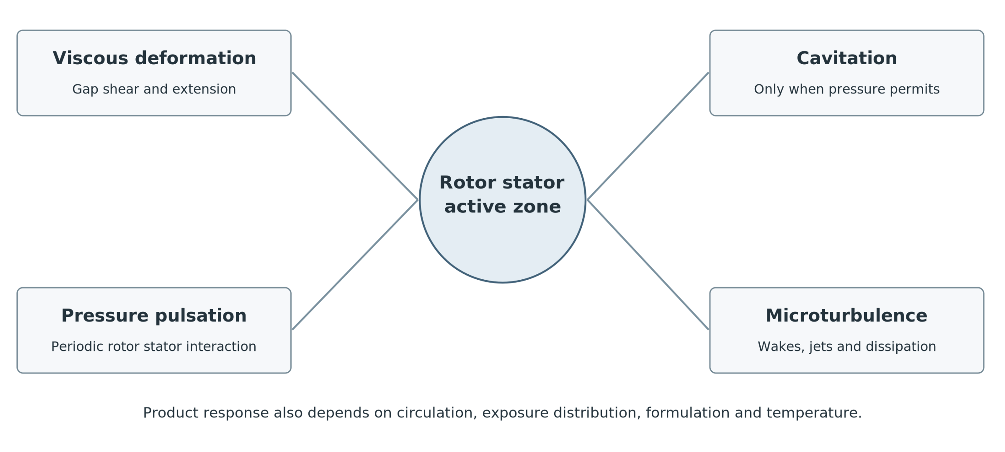
Figure 9.13. Mechanisms that may operate within the active region of a rotor-stator mixer. Their relative contributions depend on geometry, material properties, and operating conditions [1].

Table 9.1. Mechanisms of action and their characteristic observable indicators

Mechanism	Physical cause	Observable indicators	Design controls
Intense shear	High velocity gradients and extensional deformation in gaps, at edges, and within jets.	Torque, rheological response, and droplet or agglomerate breakup without cavitation noise.	Tip speed, clearance, blade shape, stator restriction, and viscosity.
Hydrodynamic cavitation	Vapor cavities form at low pressure and collapse after pressure recovery; gas nuclei alter the dynamics.	Broadband noise, vapor clouds, erosion, pressure minima, and radical formation in suitable liquids.	Absolute pressure, temperature, geometry, dissolved gas, cavitation number, and backpressure.
Pressure pulsations	Periodic rotor-stator passage with time varying open flow area.	Discrete spectral peaks at element passage frequency and its harmonics.	Element count, relative phase, opening area, speed, and housing compliance.
Small-scale turbulence	Breakdown of wakes and jets into fluctuating eddies with intermittent dissipation.	Broad velocity spectrum, rapid micromixing, and power dependent on the Reynolds number.	Reynolds number, jet velocity, hole pitch, staging, and local dissipation.
Impact and cutting	Direct contact with leading edges or hard inclusions.	Fragmentation of soft particles, edge wear, and dependence on initial particle size.	Edge profile, feed direction, particle hardness, and clearance.
Acoustic streaming	Mean flow induced by oscillations of pressure and velocity.	Secondary circulation and transport beyond a steady-flow prediction.	Amplitude, frequency, chamber geometry, and damping.

9.8 Mathematical Model Closure and Computational Validation of Hydrodynamic Processes

The analytical relations presented above form a hierarchy of descriptors and conditional models. Kinematic equations define speed scales and event frequencies; energy balances describe total power input and thermal dose; and rheological, turbulence, and cavitation models require detailed local flow conditions and constitutive closures. Final droplet or particle size distributions cannot be predicted using only bulk variables such as rotor tip speed or installed motor power. Reliable breakup and coalescence kinetic parameters, statistics of hydrodynamic exposure, and well-defined initial conditions are also required.

Computational fluid dynamics (CFD) models should first reproduce integral performance at the actual operating point, including flow rate, torque, and differential pressure. Mesh and sensitivity analyses of the time step are essential around narrow gaps and perforations. Rotor-stator phase interactions require transient techniques, such as sliding meshes. Local dissipation fields must be accompanied by the averaging volumes and time windows used to derive them. Attractive colored contours do not replace numerical validation, and turbulent dissipation predicted by a closure model must not be equated directly with locally measured stresses [3].

Lebon and colleagues compared stator perforation configurations in batch and inline high shear conditioning of metal melts. Their simulations showed that geometry optimized for local agglomerate breakup might distribute material poorly, and that predictions were sensitive to turbulence model choice [8]. This supports process specific design, but numerical coefficients and material responses determined for those media cannot be transferred directly to fundamentally different systems, such as oil-in-water emulsions.

Mathematical models should therefore be validated hierarchically at three levels:

• Global level: Verify overall equipment balances, including flow rate, pressure head, and power consumption.

• Local level: Model and corroborate the hydrodynamic mechanisms operating within the active region.

• Product level: Compare predicted process characteristics against actual properties of the finished product.

Calibrating dispersion models against only one averaged diameter can conceal compensating errors in local dissipation, residence time, and coalescence. Reliable validation of model transferability requires experiments over different rotational speeds and throughputs, complete size distributions, and a recorded thermal history.