Cavitation-Assisted Particle Dispersion

5 Hydrodynamic stress, particle response, and process models

5.1 Particle response time and inertia

A spherical particle in creeping flow has a characteristic relaxation time:

The Stokes number relative to a flow time scale ${\tau }_f$ is:

Particles with $St\ll 1$ follow liquid motion closely, while particles with larger $St$ retain inertia and can collide with other particles or surfaces. Agglomerates are porous and irregular, so Equation (5.1) is only a reference scale. The effective density and drag differ from those of a compact sphere.

5.2 Turbulent length and time scales

The Kolmogorov microscale is:

and the Kolmogorov time scale is:

where $\nu$ is kinematic viscosity and ${\epsilon }_t$ is local turbulent energy dissipation rate per unit mass. Figure 5.1 shows how the smallest turbulent length scale decreases as local dissipation increases.

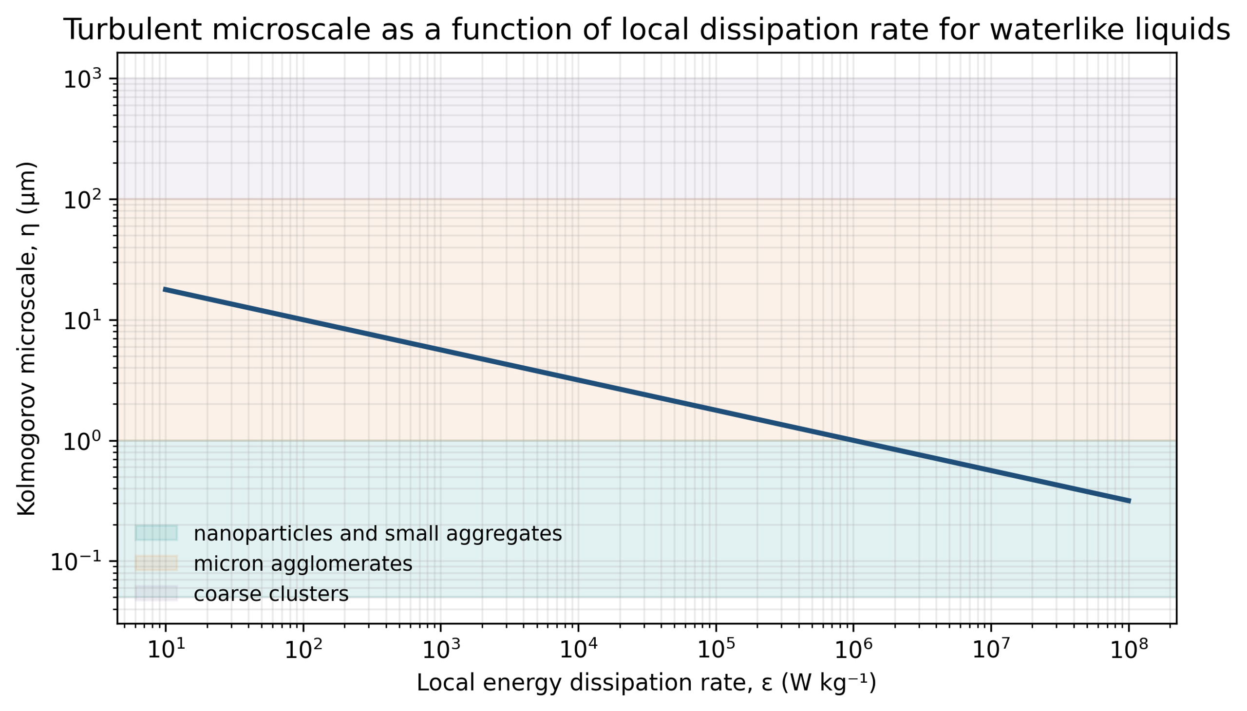
Figure 5.1. Kolmogorov microscale as a function of local energy dissipation rate for a water-like liquid. Calculation using Equation (5.3) [58].

Agglomerates smaller than ${\eta }_K$ experience an approximately linear velocity field. A viscous stress scale is:

For an agglomerate of size $d_a$ larger than ${\eta }_K$, the inertial range velocity difference is:

and the associated inertial stress scale is:

The characteristic strain rate in the smallest eddies is:

The local maximum of ${\epsilon }_t$, rather than the vessel average, determines the most severe turbulent loading. Collapse induced impulses can greatly exceed the steady turbulent stress, but they act for a much shorter duration.

5.3 Population balance

An industrial suspension contains distributions of agglomerate size, strength, morphology, and exposure. A population balance for breakage and aggregation can be written as:

The breakage and aggregation terms can be coupled with local stress exposure, residence time, and formulation dependent collision efficiency. In Equation (5.9), the aggregation operator 𝒜[n] represents the net contribution of aggregation. Mechanistic models compare agglomerate strength with hydrodynamic or collapse-induced stress, while aggregation models account for reattachment after new surface is created [14,38]. These models help distinguish gradual erosion from rapid rupture and explain why an immediate size reduction may not remain stable. High velocity interparticle collisions observed under cavitating acoustic fields provide one experimental basis for including collision terms in breakage and aggregation models [46].

5.4 Pass distribution and cumulative exposure

For a well-mixed recirculating batch, the nominal number of passes is:

where $Q$ is loop flow rate, $t$ is processing time, and $V_b$ is batch volume. A perfectly mixed tank produces a distribution of actual passes. Under an ideal Poisson approximation, the fraction that has experienced $k$ passes is:

This relation illustrates that the nominal pass number is an average. Tank stratification, short-circuiting, dead zones, and sampling location create broader distributions. A pass count should always be reported with batch volume, loop flow, loop holdup, and tank mixing arrangement.

The hydraulic power supplied across the cavitation device is:

The ideal hydraulic energy input per unit mass for one pass is:

A cumulative estimate including overall hydraulic efficiency ${\eta }_h$ is:

Equations (5.12) to (5.14) quantify pump energy, not the fraction delivered to particle breakage. Energy is also converted into heat, residual kinetic energy, sound, wall friction, bubble formation, bubble collapse, and erosion.

If all dissipated energy ultimately becomes sensible heat, the adiabatic temperature rise is approximately:

This expression provides an upper bound for a batch without cooling. In production, the heat exchanger duty should be based on measured motor power, hydraulic power, and steady state temperature.