# Cavitation-Assisted Particle Dispersion
## Abstract
Hydrodynamic cavitation provides a media-free route for particle dispersion, deagglomeration, controlled comminution, and exfoliation by combining extensional flow, viscous and turbulent stresses, bubble-induced particle motion, liquid microjets, shock waves, and high-velocity interparticle interactions. This article develops an engineering framework that links particulate structure, colloidal stability, cavitation dynamics, local stress scales, cumulative exposure, and process equipment to measurable product attributes. The analysis distinguishes reversible deagglomeration from aggregate or primary-particle fracture and emphasizes control of the coarse tail of the particle-size distribution, rheology, morphology, crystal structure, chemical purity, and aged stability. Quantitative case studies covering metal oxides, silver, nanofluids, pharmaceuticals, soy slurries, silicon, graphite, carbon nanotubes, resins, and plant raw materials demonstrate strong first-pass effects, formulation-dependent endpoints, and the risk of overprocessing. Practical scale-up is based on preserving critical pressure history and passage geometry, controlling residence-time and pass distributions, managing heat and erosion, and increasing throughput by parallelization or staged processing. The appropriate endpoint is therefore the minimum cavitation severity and cumulative exposure that achieve a stable particle-size distribution while preserving the properties required by the final application.
## 1 Introduction
Common hydraulic definitions, energy boundaries, residence-time expressions, uncertainty requirements, and scale-translation principles are consolidated in Section 6.2. The present article adopts that framework and develops the mechanisms, models, and acceptance criteria specific to cavitation-assisted particle dispersion.
Particle dispersion and deagglomeration are critical operations in the manufacture of catalysts, ceramic slips, electronic inks and pastes, battery suspensions, nanofluids, pharmaceutical formulations, pigments, coatings, polymer composites, thermal-interface materials, food slurries, and two-dimensional materials. The engineering objective is not simply to reduce an instrument-reported diameter. A successful process must generate a reproducible dispersed-particle population, control the coarse tail of the particle-size distribution, preserve the required morphology and crystal structure, and maintain chemical stability at newly created solid-liquid interfaces.
Hydrodynamic cavitation provides a distinctive combination of mechanical stresses for these purposes. Acceleration through a restriction or a rapidly varying flow field can lower local static pressure sufficiently to generate vapor or gas-filled cavities. The cavities grow, convect, interact with suspended solids, and collapse during pressure recovery. Collapse produces pressure pulses, shock waves, liquid microjets, intense velocity gradients, turbulent dissipation, and rapid particle acceleration. In combination, these effects can separate weak agglomerates, erode aggregate surfaces, fracture brittle crystals, exfoliate layered materials, remove attached contaminants, and modify the collision history of suspended particles [1,3,7,8,14].
Cavitation is not beneficial under all operating conditions. Excessive exposure can fracture primary particles, shorten fibers, reduce flake aspect ratio, remove functional coatings, alter crystal structure, accelerate equipment wear, increase bulk temperature, or promote reaggregation after new surfaces are formed. Cavitation has also increased the coarse-particle population in chemically sensitive chemical mechanical planarization slurries [37]. Process development must therefore control the cavitation field, particle mechanics, suspension rheology, surface chemistry, residence-time distribution, temperature, gas content, and downstream handling as coupled variables.
This article presents an engineering framework for hydrodynamic cavitation-assisted particle processing. It distinguishes deagglomeration from comminution, describes the physical and colloidal mechanisms that control dispersion, summarizes the principal governing relations, compares equipment configurations, reviews analytical methods and quantitative case studies, and provides procedures for scale-up and troubleshooting.
## 2 Particle structure and process objectives
### 2.1 Primary particles, aggregates, agglomerates, and flocs
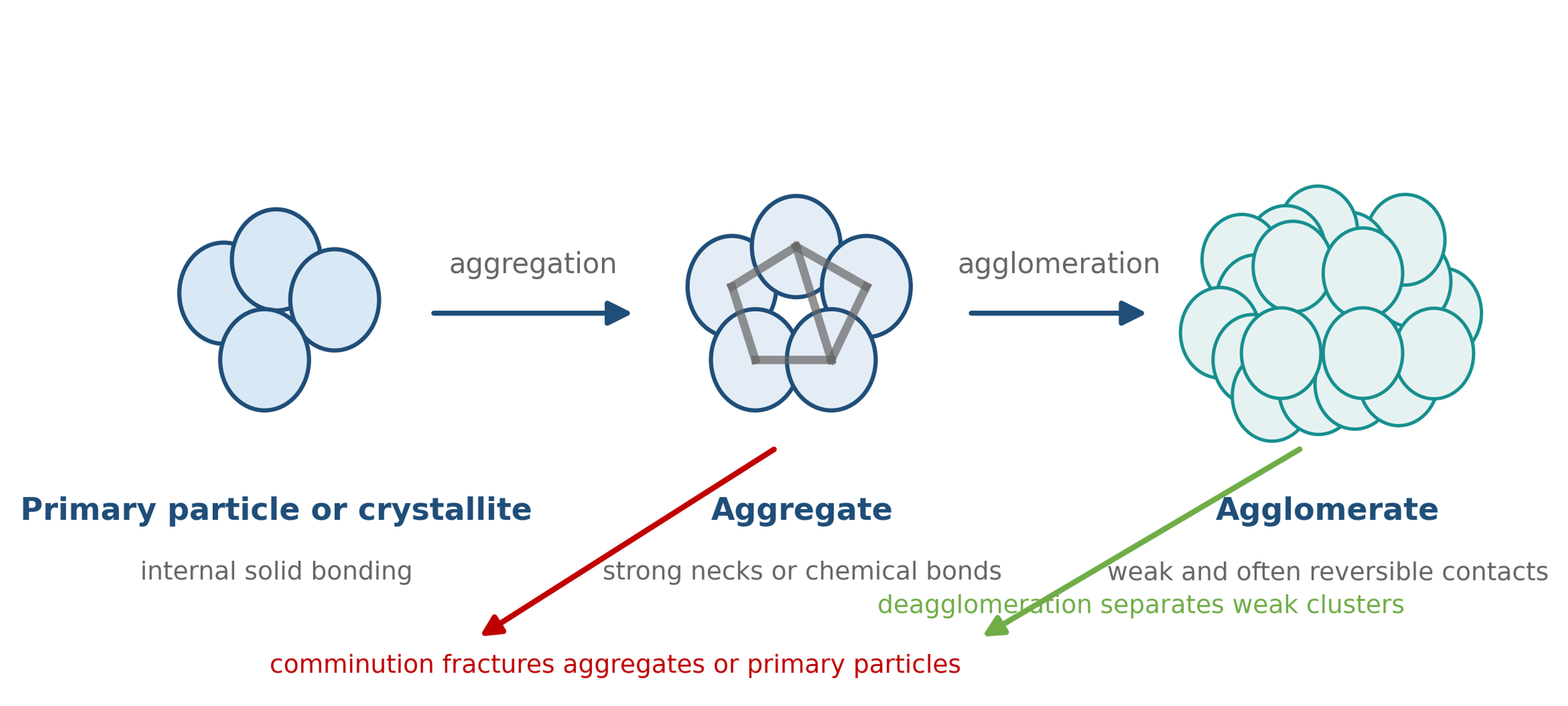
The terms primary particle, crystallite, aggregate, agglomerate, and floc describe distinct levels of particulate structure. Although these terms are often used inconsistently, the distinction determines the stress required for breakup and the interpretation of particle-size data.
A primary particle is the smallest discrete solid object relevant to the process. It may be a single crystal, a polycrystalline grain, a platelet, a flake, a fiber, a hollow sphere, or an irregular fragment. Crystallite is a coherent diffraction domain and may be smaller than a polycrystalline primary particle. An aggregate consists of primary particles joined by strong necks, sintered contacts, covalent bonds, siloxane bonds, or other contacts that are not readily reversible in the liquid. An agglomerate is a larger cluster held mainly by weaker van der Waals attraction, capillary bridges, electrostatic attraction, polymer bridging, or mechanical interlocking. A floc is a reversible network formed in the liquid after particles interact through attractive surface forces or bridging molecules [14,15,18,20].
Figure 2.1. Hierarchy of particulate structures and the distinction between deagglomeration and comminution [58]Source: Kozyuk O. Hydrodynamic Cavitation. Unpublished technical manuscript and supporting data, 2026.
*[Figure 2.1](#figure-2-1). Hierarchy of particulate structures and the distinction between deagglomeration and comminution [58].*
Table 2.1 summarizes the expected response of each structural level. Deagglomeration should separate weak clusters while preserving aggregates and primary particles whenever possible. Fracture of an aggregate or primary particle constitutes comminution. Exfoliation is a special case in which weak interlayer contacts are separated while the structure within each plane is preserved.
*Table 2.1. Structural hierarchy and desired cavitation response.*
| **Structure** | **Typical bonding** | **Preferred process response** | **Essential analytical evidence** |
|---------------------------------|----------------------------------------------------------------------------------------|-------------------------------------------------------|-------------------------------------------------------------------|
| Primary particle or crystallite | Internal crystal or solid state bonding | Preserve unless milling is intended | High resolution SEM or TEM, X ray diffraction, Raman spectroscopy |
| Aggregate | Sintered necks, covalent bonds, strong hydrogen bonding | Preserve or partially erode only when required | SEM or TEM, specific surface area, crystallite size |
| Agglomerate | van der Waals attraction, capillary bridges, polymer bridging, mechanical interlocking | Separate into smaller aggregates or primary particles | Laser diffraction or DLS combined with microscopy |
| Floc | Reversible network formed in the liquid | Break the network and reduce yield stress | Rheometry, microscopy, sedimentation behavior |
| Layered stack or tactoids | Weak interlayer attraction | Delaminate or exfoliate while preserving lateral size | AFM or TEM thickness, Raman response, diffraction |
### 2.2 Particle size distribution and top size control
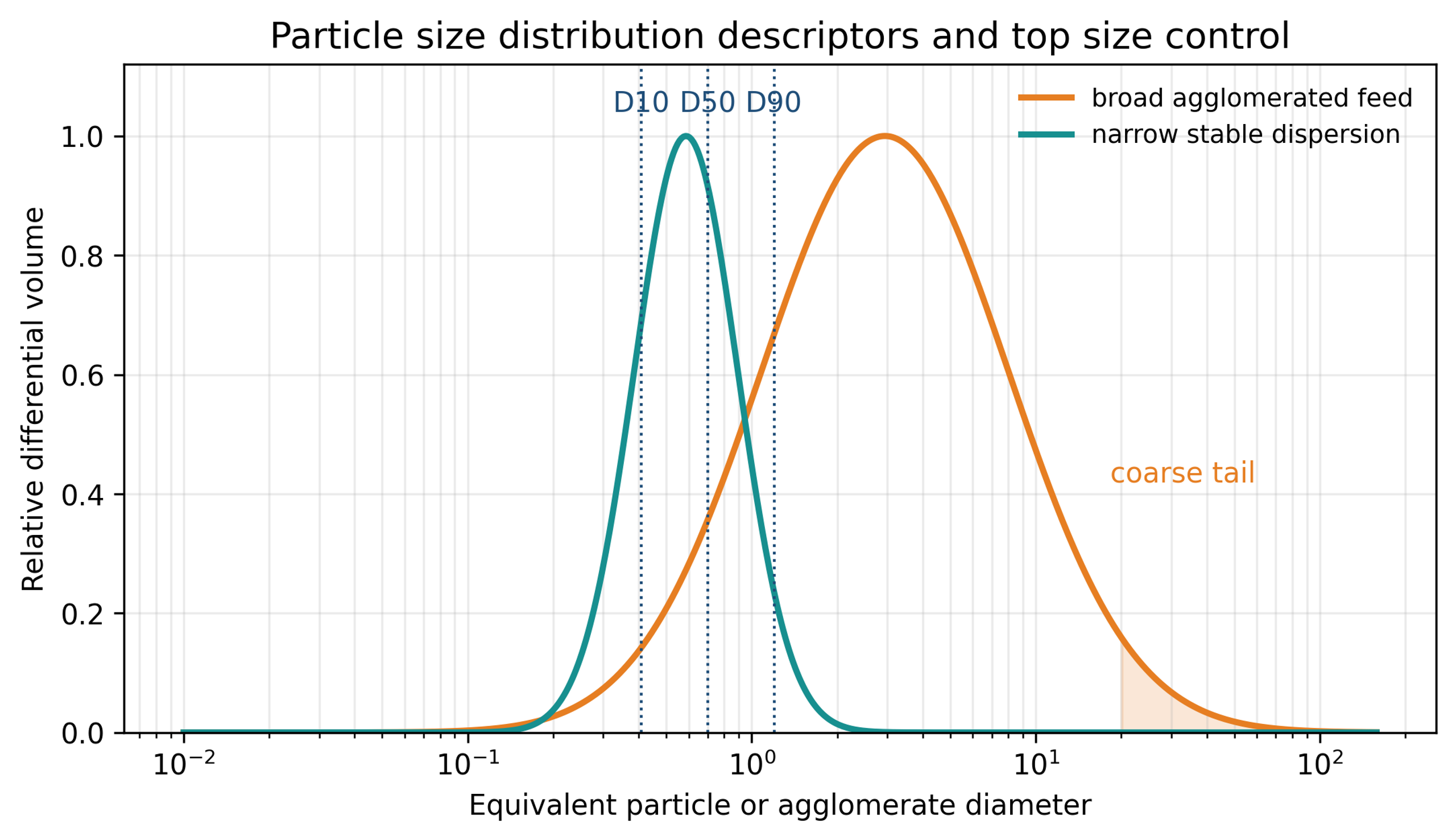
A single mean diameter is rarely sufficient to specify a dispersion. The percentiles , , and define the diameters below which 10, 50, and 90 percent of the specified distribution fall. The distribution basis must be reported because number-weighted, surface-weighted, and volume-weighted distributions emphasize different parts of the population. Laser diffraction normally reports a volume-based equivalent diameter. Dynamic light scattering is strongly biased toward larger scatterers and reports a hydrodynamic diameter. Microscopy provides a direct view of particle shape and clustering but examines a smaller population.
Figure 2.2. Particle size distribution descriptors and the importance of the coarse tail [58]Source: Kozyuk O. Hydrodynamic Cavitation. Unpublished technical manuscript and supporting data, 2026.
*[Figure 2.2](#figure-2-2). Particle size distribution descriptors and the importance of the coarse tail [58].*
The width of a volume-based distribution is often summarized by the span:
(2.1)
A low span indicates a narrow distribution, but a narrow distribution is not necessarily stable. The same sample should be measured immediately after processing and after a defined aging period. A reduction in combined with an unchanged or increased may indicate that most agglomerates were dispersed while a small resistant population or contaminant population remained. For printing, coating, filtration, and electronic applications, or a direct coarse particle count can be more important than the mean.
The percent reduction in a selected size metric is:
(2.2)
where is the reduction in percent. This calculation is meaningful only when the analytical method, optical properties, dispersion procedure, solids concentration, and sampling protocol remain consistent.
### 2.3 Product specifications
A cavitation dispersion process should be defined through measurable critical quality attributes rather than pressure or pass count alone. Typical targets include:
- , , , span, and a specified maximum particle count.
- Viscosity, yield stress, thixotropic recovery, and flow behavior at the required solids loading.
- Sedimentation, creaming, or phase separation during storage and transport.
- Preservation of crystal phase, surface treatment, particle shape, aspect ratio, and porosity.
- Chemical purity, especially metals released by pump, valve, and reactor wear.
- Acceptable temperature rise, gas entrainment, foam, and solvent loss.
- Throughput, cleaning time, batch repeatability, and energy consumption.
- Functional properties such as conductivity, thermal conductivity, opacity, catalytic activity, dissolution rate, or mechanical strength.
Table 2.2 illustrates how the controlling specification changes with the application.
*Table 2.2. Representative product objectives for cavitation dispersed materials.*
| **Application** | **Primary particle objective** | **Critical upper tail concern** | **Additional performance test** |
|---------------------------|--------------------------------------------------------------|------------------------------------------|------------------------------------------------------------|
| Conductive silver ink | Separate powder or flake clusters without excessive fracture | Screen blockage and printed line defects | Electrical resistivity, printability, cured microstructure |
| Ceramic slip | Break tactoids and reduce viscosity | Surface defects and nozzle blockage | Casting density, shrinkage, fired microstructure |
| Nanofluid | Reduce hydrodynamic agglomerate size | Sedimentation and channel blockage | Aged size, thermal conductivity, viscosity |
| Pharmaceutical suspension | Reduce crystals or agglomerates to a controlled range | Dose nonuniformity and poor dissolution | Polymorph, dissolution, chemical stability |
| Fiber filled polymer | Separate fiber bundles | Unmixed bundles and local defects | Fiber length, conductivity, mechanical properties |
| Layered material | Exfoliate stacks to thin sheets | Thick unexfoliated platelets | Sheet thickness, lateral size, defect density |
| Food or biomass slurry | Disrupt cells and reduce coarse fragments | Grit, mouthfeel, fouling | Rheology, extractability, sensory or separation behavior |
## 3 Colloidal forces, agglomerate strength, and suspension stability
### 3.1 Interparticle attraction and stabilization
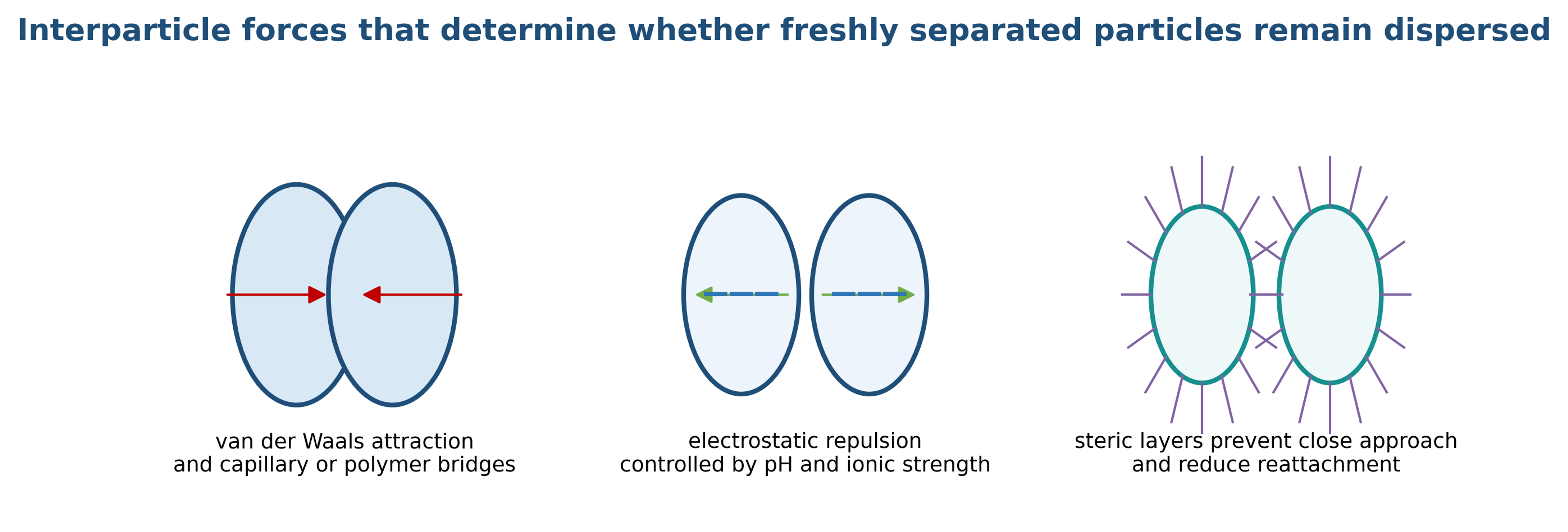
Deagglomeration increases the solid-liquid interfacial area. The mechanical process is therefore inseparable from formulation chemistry. A cluster separated in the collapse zone may reattach within milliseconds unless the liquid provides sufficient electrostatic, steric, or electrosteric stabilization.
Figure 3.1. Principal interparticle forces that determine whether freshly separated particles remain dispersed [58]Source: Kozyuk O. Hydrodynamic Cavitation. Unpublished technical manuscript and supporting data, 2026.
*[Figure 3.1](#figure-3-1). Principal interparticle forces that determine whether freshly separated particles remain dispersed [58].*
For two particles, the total interaction potential is commonly represented as the sum of van der Waals attraction, electrostatic repulsion, steric interaction, and any additional nonideal contribution:
(3.1)
For two equal spheres of radius at a small surface separation , a useful approximation for van der Waals attraction is:
(3.2)
where is the Hamaker constant. The corresponding attractive force scale is:
(3.3)
Electrostatic repulsive interaction depends on surface potential, ion valence, and ionic strength. For a symmetric electrolyte and moderate surface potential, a simplified constant potential expression for two spheres is:
(3.4)
The Debye screening length is:
(3.5)
where is ionic strength. Increasing ionic strength reduces the screening length and can cause rapid aggregation even when immediate particle size after cavitation is small. Zeta potential is useful for comparing related electrostatic systems, but it is not a universal stability criterion. Sterically stabilized systems may remain stable at low zeta potential because adsorbed polymer layers prevent close approach.
Capillary bridges can dominate dry powder agglomeration and partially wetted feed systems. A simple capillary force scale is:
(3.6)
where is liquid surface tension and is the contact angle. Complete wetting and removal of trapped gas can reduce capillary cohesion, although rapid cavitation may also introduce additional gas-liquid interfaces.
For approximately spherical nonporous particles, the external area per unit mass is:
(3.7)
The increase in surface area after deagglomeration can sharply increase dispersant demand. The first estimate of dispersant mass is:
(3.8)
where is the adsorbed mass per unit area and is the mass of solid. Equation (3.8) is a formulation estimate, not a substitute for an adsorption isotherm. Excess polymer may increase viscosity or cause bridging flocculation, while insufficient polymer permits reattachment.
### 3.2 Agglomerate strength
Agglomerate failure occurs when external stress exceeds a local strength that depends on bond force, coordination number, porosity, primary particle size, and defect structure. A generalized contact network strength relation is:
(3.9)
where is agglomerate tensile strength, is a structural coefficient, is agglomerate porosity, is a characteristic bond force, and is the size of the load bearing building block [14–16]. Real agglomerates have a distribution of bond strengths. Weak outer branches may erode gradually while a compact core remains intact. Strong impulses may split a cluster into several daughter fragments. Repeated subcritical impulses can also produce fatigue-like erosion.
A useful local breakage number is:
(3.10)
where is an applied hydrodynamic or collapse-induced stress. Values below unity indicate that instantaneous rupture is unlikely, although repeated loading may still erode the structure. Values substantially above unity favor rapid rupture or shattering. The fragment distribution cannot be predicted from alone.
### 3.3 Sedimentation, Brownian motion, and rheology
Dispersion can meet an immediate particle-size target and still fail during storage. For an isolated spherical particle in the Stokes regime, the terminal settling velocity is:
(3.11)
The Brownian diffusion coefficient is:
(3.12)
A sedimentation Peclet number over a characteristic height is:
(3.13)
Large indicates that gravity dominates Brownian redistribution. Equations (3.11) to (3.13) are screening relations. Concentrated suspensions exhibit hindered settling, network formation, yield stress, and non-Newtonian flow. Deagglomeration often increases wetted surface area and may increase viscosity if dispersant is insufficient. In other systems, breakup of a space-spanning floc network reduces yield stress and viscosity. Rheology is therefore an independent response, not a predictable consequence of a smaller median diameter [20].
## 4 Cavitation physics and bubble particle interaction
### 4.1 Cavitation inception and pressure history
Hydrodynamic cavitation begins when local pressure approaches a threshold controlled by vapor pressure, dissolved gas, nuclei population, liquid tensile strength, surface roughness, and flow history. A commonly used cavitation number is:
(4.1)
where is a reference or recovered pressure, is saturation vapor pressure, and is a characteristic velocity. Lower values generally indicate stronger cavitation, but the inception value is specific to geometry and nuclei condition [3,21,22].
For an ideal pressure conversion through a restriction, a velocity scale is:
(4.2)
where is a discharge coefficient and is pressure drop. Equation (4.2) does not describe the complete multiphase field, but it shows why pressure drop strongly affects velocity, strain rate, and collapse intensity.
The radial motion of an isolated spherical bubble is described by the Rayleigh-Plesset equation. Classical treatments of cavitation and bubble oscillation provide the basis for this relation [4-6].
(4.3)
A polytropic approximation for the noncondensable gas pressure is:
(4.4)
where *k* is the polytropic exponent. For an empty spherical cavity that collapses from an initial radius . For a constant far field pressure difference, Equation (4.5) gives Rayleigh collapse time. The relation follows Rayleigh’s classical analysis [47].
(4.5)
These equations establish important trends but do not directly predict an industrial bubble cloud. In a cavitating restriction, bubbles interact with neighboring bubbles, particles, walls, turbulence, dissolved gas, and changing pressure. Cloud collapse can redistribute energy and shield inner bubbles.
### 4.2 Interaction stages
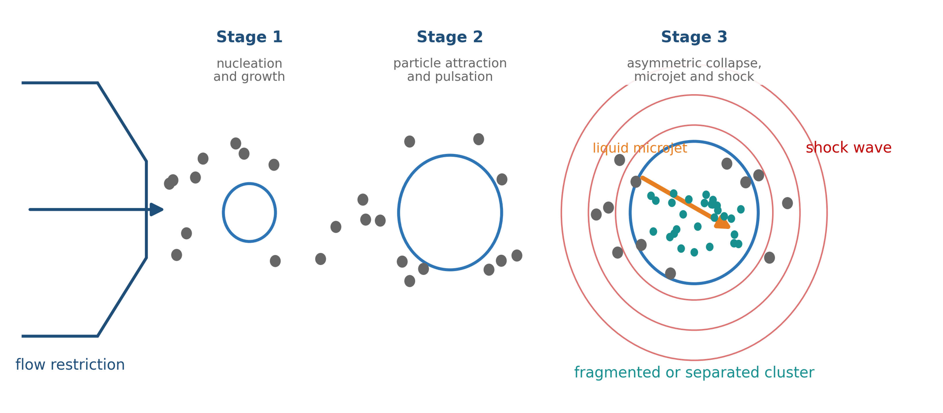
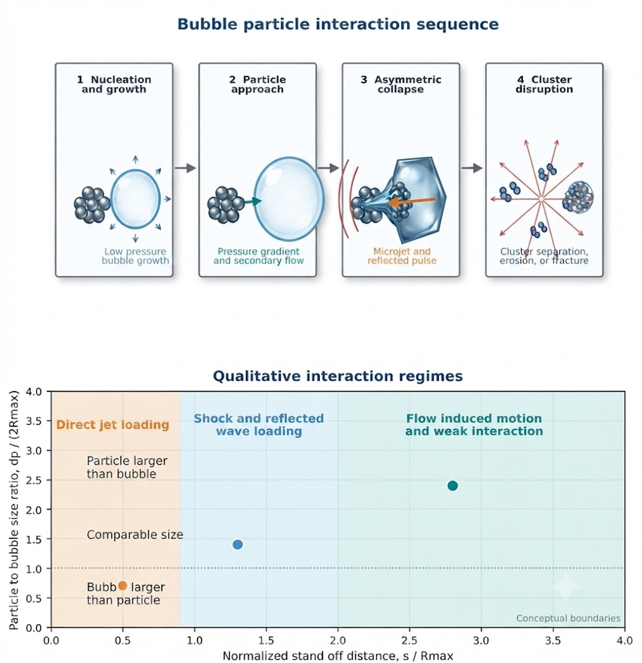
The interaction between a bubble and suspended particles can be divided into three overlapping stages. During nucleation and growth, the bubble displaces liquid and modifies particle trajectories. During pulsation and convection, secondary pressure forces and local recirculation can concentrate particles near the bubble interface. During asymmetric collapse, a liquid microjet forms and a pressure pulse propagates into the surrounding suspension.
Figure 4.1. Conceptual stages of interaction between cavitation bubbles and suspended particles [8–10,41,42]Original diagram based on Yu et al. (2024), Wolfrum et al. (2003), Borkent et al. (2008), Arora et al. (2004), and Poulain et al. (2015).
*[Figure 4.1](#figure-4-1). Conceptual stages of interaction between cavitation bubbles and suspended particles.*
Bubble particle interaction depends strongly on bubble standoff distance, particle size relative to bubble size, particle density, surface wettability, and the recovered pressure gradient. Particles may accelerate away from a growing bubble and then move toward the collapse region. Controlled experiments have reported particle velocities spanning orders of magnitude because only a small fraction of particles intercept the most intense jet or collapse zone [10,41,42].
### 4.3 Microjets, shock waves, and particle loading
A bubble that collapses near a solid surface or particle generally becomes nonspherical. The side farther from the boundary accelerates toward the near side and forms a high-velocity liquid microjet. The jet penetrates the bubble and strikes the opposite interface or a nearby solid. At the same time, rapid liquid deceleration emits an outward pressure pulse. Studies show that wall or particle proximity strongly alters collapse symmetry, jet direction, and pressure transmission [8,45]. Related acoustic cavitation studies show that shock loading from collapse can fragment molecular crystals, while wall shear and collapse near a surface can remove attached material [12,13,43,44].
The peak pressure transmitted from a liquid jet into a solid can be estimated by acoustic impedance matching:
(4.6)
where and are sound speeds, and are densities, and is jet velocity. If the solid acoustic impedance greatly exceeds that of the liquid,
(4.7)
A related semiempirical stress scale used in agglomerate dispersion models is:
(4.8)
where is an empirical transfer coefficient [14]. These relations are scaling estimates. The stress reaching a particle depends on wave geometry, attenuation, cloud shielding, orientation, impedance mismatch, and whether the particle lies in the jet path.
Experiments and simulations show that the interaction regime changes with standoff distance and the particle to bubble size ratio. Close particles promote asymmetric collapse and direct jet loading; at larger separation, reflected pressure waves and flow-induced particle motion become more important [8,11].
Figure 4.2. Bubble particle interaction stages and qualitative regimes as functions of normalized standoff distance and particle-to-bubble size ratio [58]Source: Kozyuk O. Hydrodynamic Cavitation. Unpublished technical manuscript and supporting data, 2026.
*[Figure 4.2](#figure-4-2). Bubble particle interaction stages and qualitative regimes as functions of normalized standoff distance and particle-to-bubble size ratio [58].*
### 4.4 Spatial separation of stress mechanisms
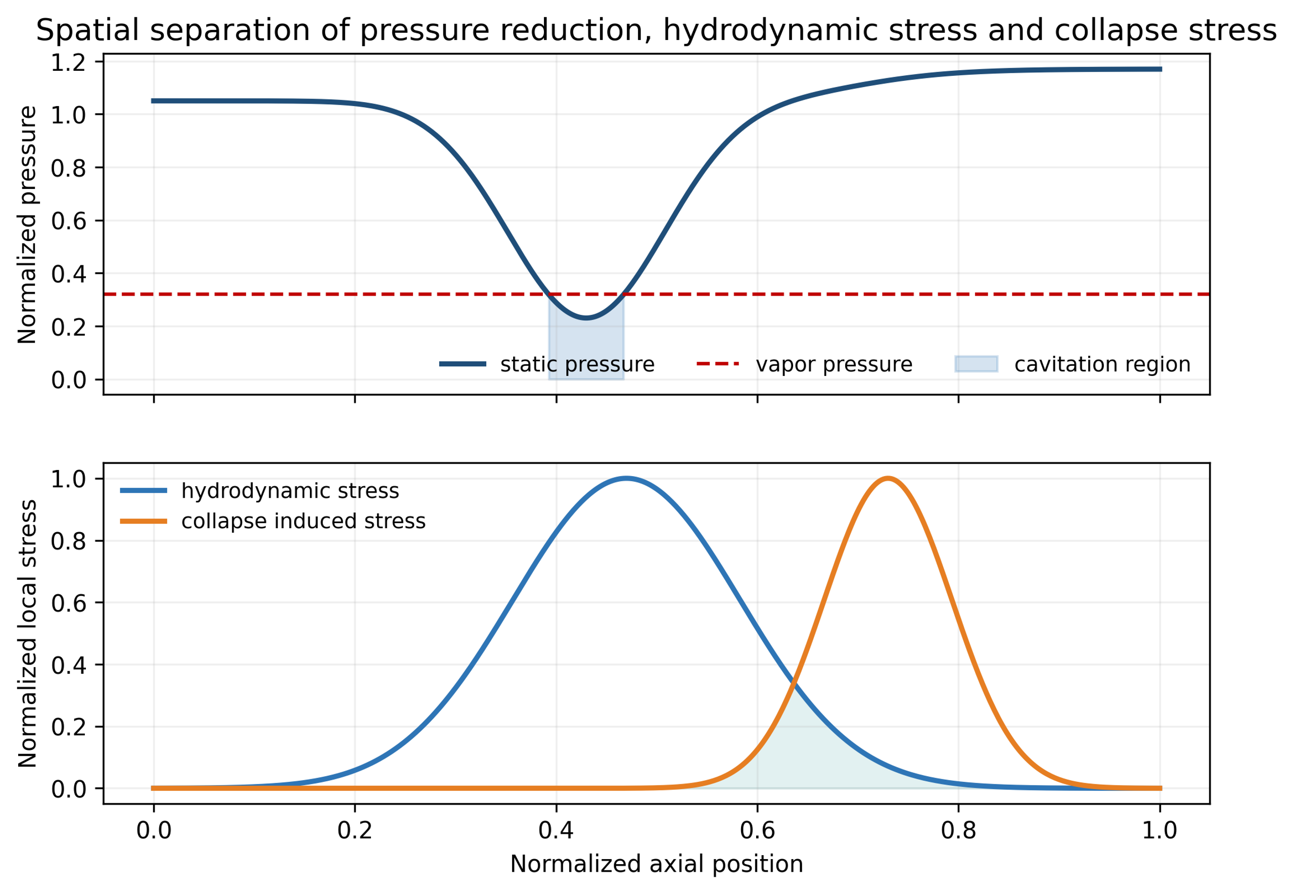
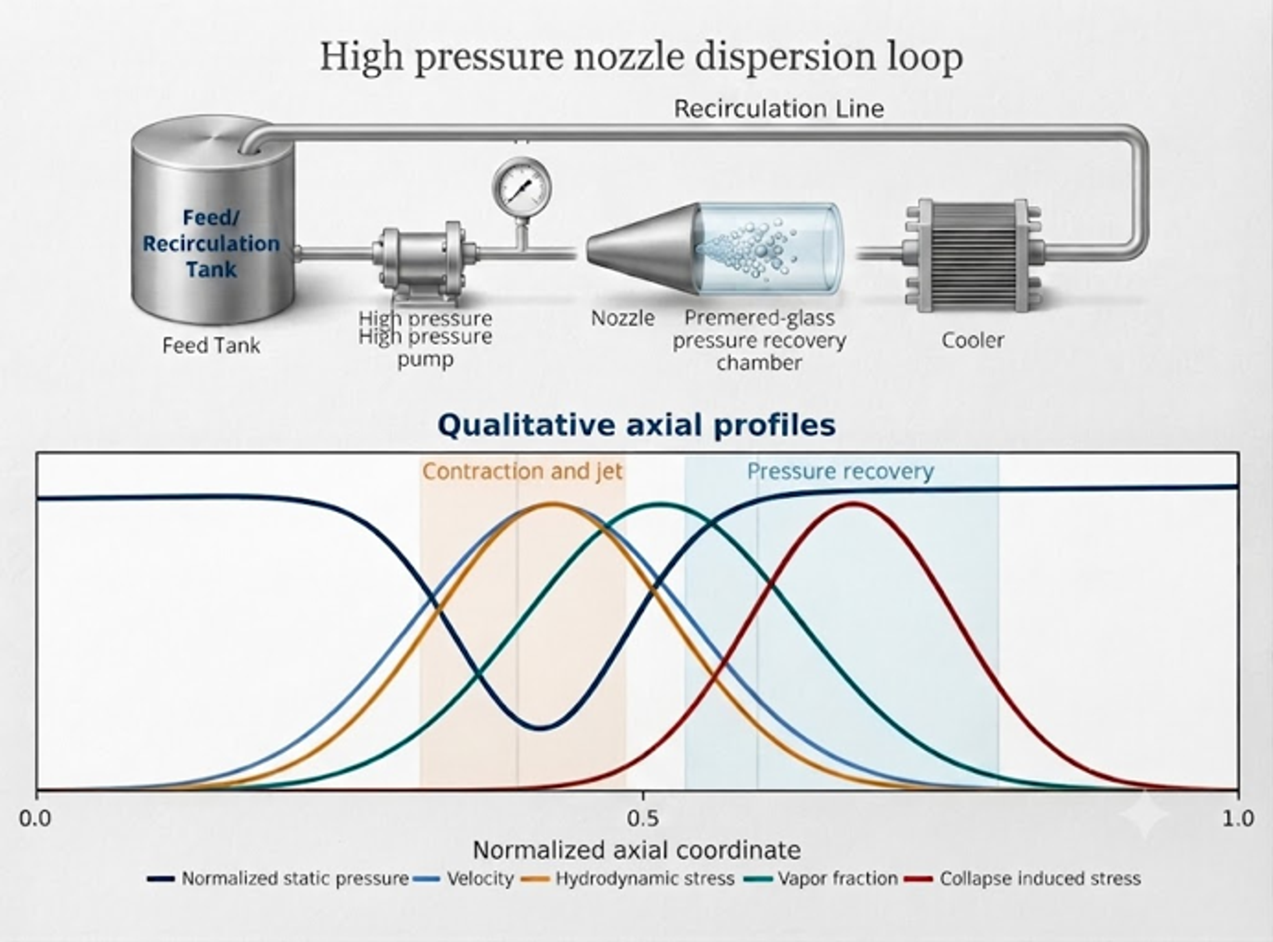
Hydrodynamic cavitation equipment creates several stress zones. Extensional acceleration is strongest near a contraction. Viscous shear acts in boundary layers and narrow passages. Turbulent stress develops in the emerging jet and mixing chamber. Collapse induced stress becomes strongest during pressure recovery. The dominant particle response depends on where the particle is located relative to these zones.
Figure 4.3. Conceptual axial pressure and stress distributions through a cavitating restriction [58]Source: Kozyuk O. Hydrodynamic Cavitation. Unpublished technical manuscript and supporting data, 2026.
*[Figure 4.3](#figure-4-3). Conceptual axial pressure and stress distributions through a cavitating restriction [58].*
The separation shown in [Figure 4.3](#figure-4-3) explains why pressure drop or average power density alone cannot uniquely predict particle-size reduction. Two devices with the same pressure drop may create different cavity lengths, recovery gradients, jet spreading rates, and collapse locations.
## 5 Hydrodynamic stress, particle response, and process models
### 5.1 Particle response time and inertia
A spherical particle in creeping flow has a characteristic relaxation time:
(5.1)
The Stokes number relative to a flow time scale is:
(5.2)
Particles with follow liquid motion closely, while particles with larger retain inertia and can collide with other particles or surfaces. Agglomerates are porous and irregular, so Equation (5.1) is only a reference scale. The effective density and drag differ from those of a compact sphere.
### 5.2 Turbulent length and time scales
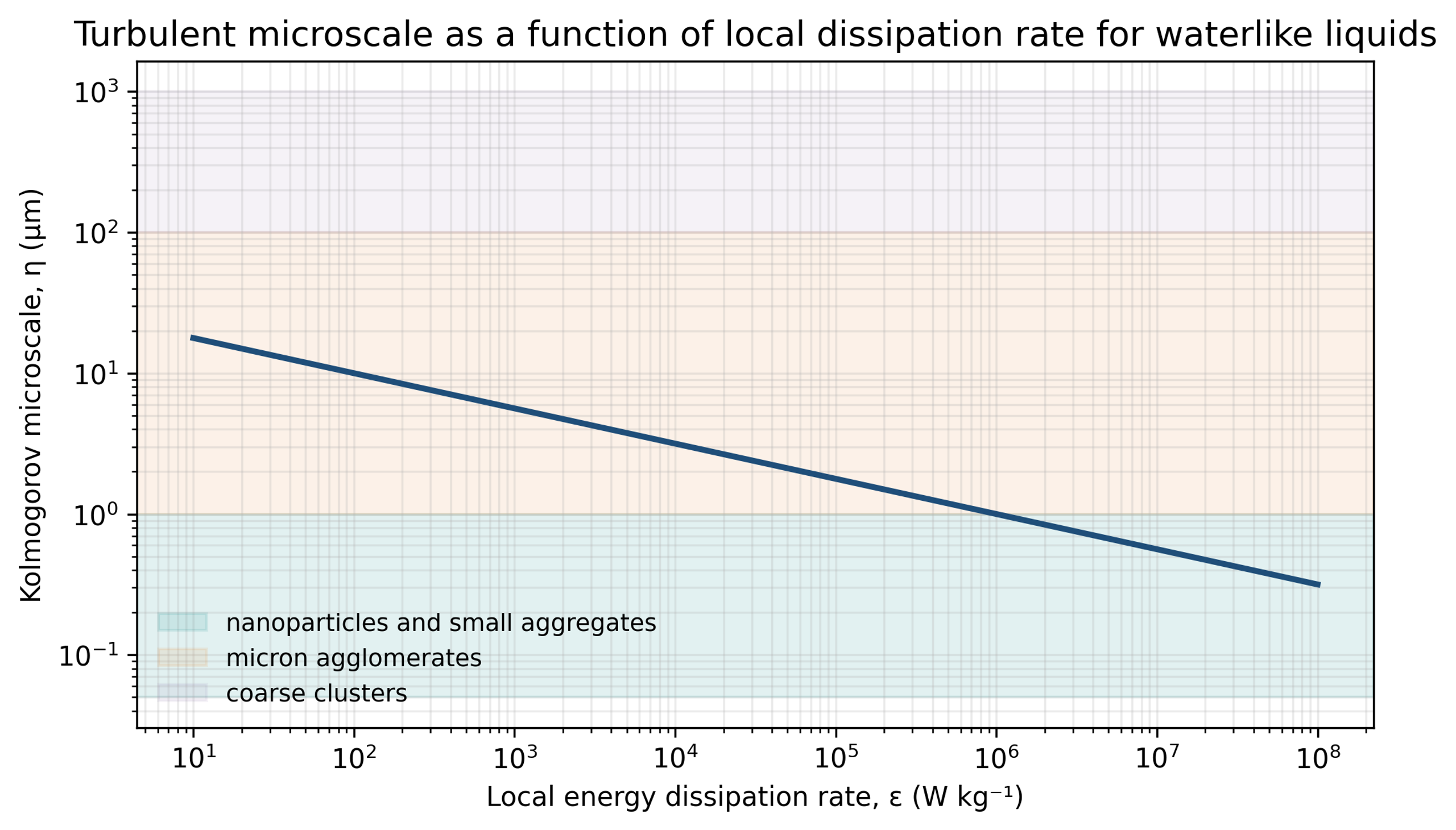
The Kolmogorov microscale is:
(5.3)
and the Kolmogorov time scale is:
(5.4)
where is kinematic viscosity and is local turbulent energy dissipation rate per unit mass. [Figure 5.1](#figure-5-1) shows how the smallest turbulent length scale decreases as local dissipation increases.
Figure 5.1. Kolmogorov microscale as a function of local energy dissipation rate for a water-like liquid. Calculation using Equation (5.3) [58]Source: Kozyuk O. Hydrodynamic Cavitation. Unpublished technical manuscript and supporting data, 2026.
*[Figure 5.1](#figure-5-1). Kolmogorov microscale as a function of local energy dissipation rate for a water-like liquid. Calculation using Equation (5.3) [58].*
Agglomerates smaller than experience an approximately linear velocity field. A viscous stress scale is:
(5.5)
For an agglomerate of size larger than , the inertial range velocity difference is:
(5.6)
and the associated inertial stress scale is:
(5.7)
The characteristic strain rate in the smallest eddies is:
(5.8)
The local maximum of , rather than the vessel average, determines the most severe turbulent loading. Collapse induced impulses can greatly exceed the steady turbulent stress, but they act for a much shorter duration.
### 5.3 Population balance
An industrial suspension contains distributions of agglomerate size, strength, morphology, and exposure. A population balance for breakage and aggregation can be written as:
(5.9)
The breakage and aggregation terms can be coupled with local stress exposure, residence time, and formulation dependent collision efficiency. In Equation (5.9), the aggregation operator 𝒜[n] represents the net contribution of aggregation. Mechanistic models compare agglomerate strength with hydrodynamic or collapse-induced stress, while aggregation models account for reattachment after new surface is created [14,38]. These models help distinguish gradual erosion from rapid rupture and explain why an immediate size reduction may not remain stable. High velocity interparticle collisions observed under cavitating acoustic fields provide one experimental basis for including collision terms in breakage and aggregation models [46].
### 5.4 Pass distribution and cumulative exposure
For a well-mixed recirculating batch, the nominal number of passes is:
(5.10)
where is loop flow rate, is processing time, and is batch volume. A perfectly mixed tank produces a distribution of actual passes. Under an ideal Poisson approximation, the fraction that has experienced passes is:
(5.11)
This relation illustrates that the nominal pass number is an average. Tank stratification, short-circuiting, dead zones, and sampling location create broader distributions. A pass count should always be reported with batch volume, loop flow, loop holdup, and tank mixing arrangement.
The hydraulic power supplied across the cavitation device is:
(5.12)
The ideal hydraulic energy input per unit mass for one pass is:
(5.13)
A cumulative estimate including overall hydraulic efficiency is:
(5.14)
Equations (5.12) to (5.14) quantify pump energy, not the fraction delivered to particle breakage. Energy is also converted into heat, residual kinetic energy, sound, wall friction, bubble formation, bubble collapse, and erosion.
If all dissipated energy ultimately becomes sensible heat, the adiabatic temperature rise is approximately:
(5.15)
This expression provides an upper bound for a batch without cooling. In production, the heat exchanger duty should be based on measured motor power, hydraulic power, and steady state temperature.
## 6 Cavitation equipment for particle processing
### 6.1 General classification
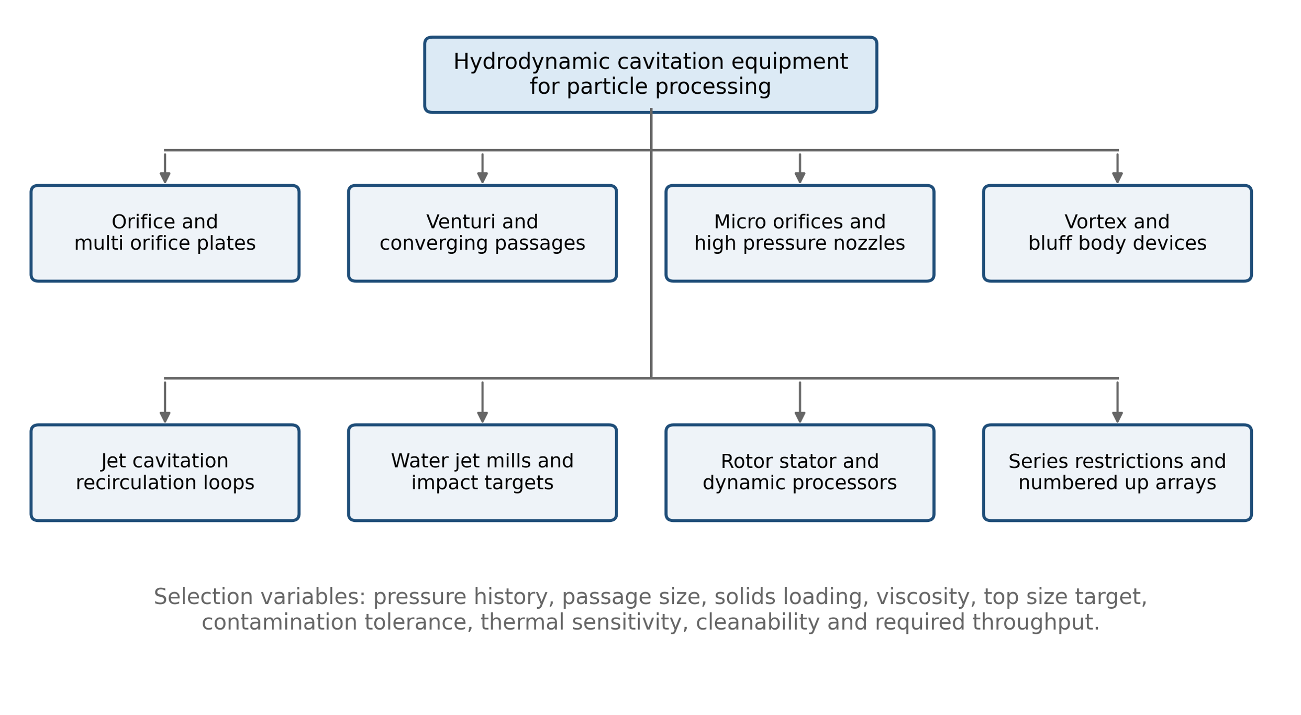
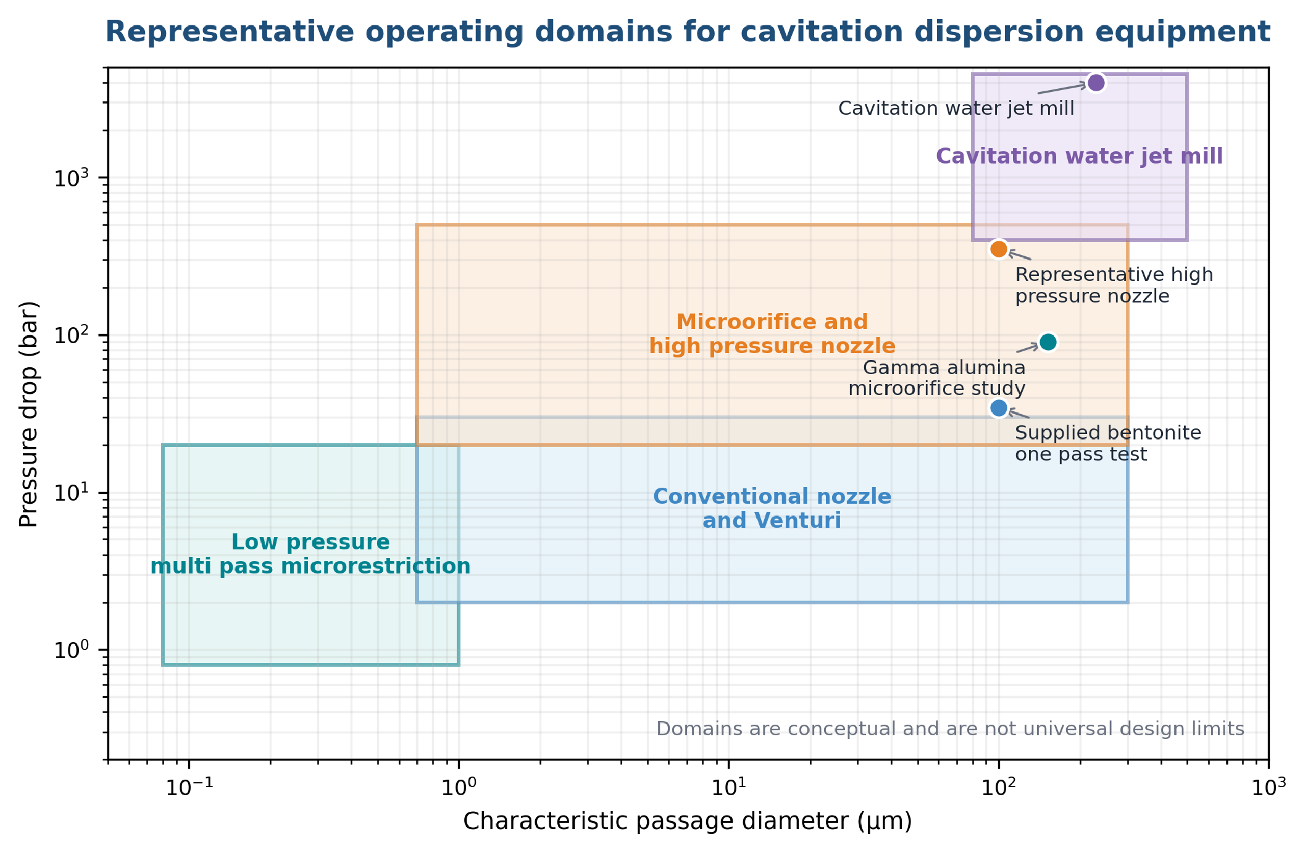
Particle processing devices range from simple orifice plates to high-pressure micron-scale nozzles and dynamic rotor stator processors. The equipment determines the pressure history, bubble cloud structure, residence time in the collapse region, exposure uniformity, erosion risk, and scale-up method.
Figure 6.1. Classification of hydrodynamic cavitation equipment used for particle dispersion and deagglomeration [58]Source: Kozyuk O. Hydrodynamic Cavitation. Unpublished technical manuscript and supporting data, 2026.
*[Figure 6.1](#figure-6-1). Classification of hydrodynamic cavitation equipment used for particle dispersion and deagglomeration [58].*
*Table 6.1. Comparison of equipment classes.*
| **Equipment class** | **Principal advantage** | **Main limitation** | **Suitable applications** |
|--------------------------------|--------------------------------------------------------|-------------------------------------------------|-----------------------------------------------------------------|
| Orifice or multi orifice plate | Simple, inexpensive, scalable, replaceable | Broad exposure distribution, plugging, erosion | Low to moderate viscosity slurries and multiple pass treatment |
| Venturi | Controlled pressure recovery and lower permanent loss | Geometry specific inception and long cavities | Continuous processing where energy recovery matters |
| Micro orifice or microchannel | High acceleration and precise passage size | Fouling, plugging, limited flow per channel | Dilute nanofluids and fine particle systems |
| High pressure nozzle | Very high velocity and stress in one pass | Pump cost, nozzle wear, temperature rise | Difficult nanoparticle agglomerates and narrow top size targets |
| Jet cavitation loop | Modular generators, recirculation, cooling | Pass distribution must be controlled | Exfoliation, comminution, pilot and production loops |
| Water jet mill | Combines cavitation, shear, impact, and classification | High pressure and complex solids handling | Brittle particles and intentional nanomilling |
| Dynamic rotor stator processor | High throughput and tolerance for viscous liquids | Mechanical seals, gap wear, scale up complexity | Production processing and concentrated formulations |
### 6.2 Orifices, Venturis, and vortex chambers
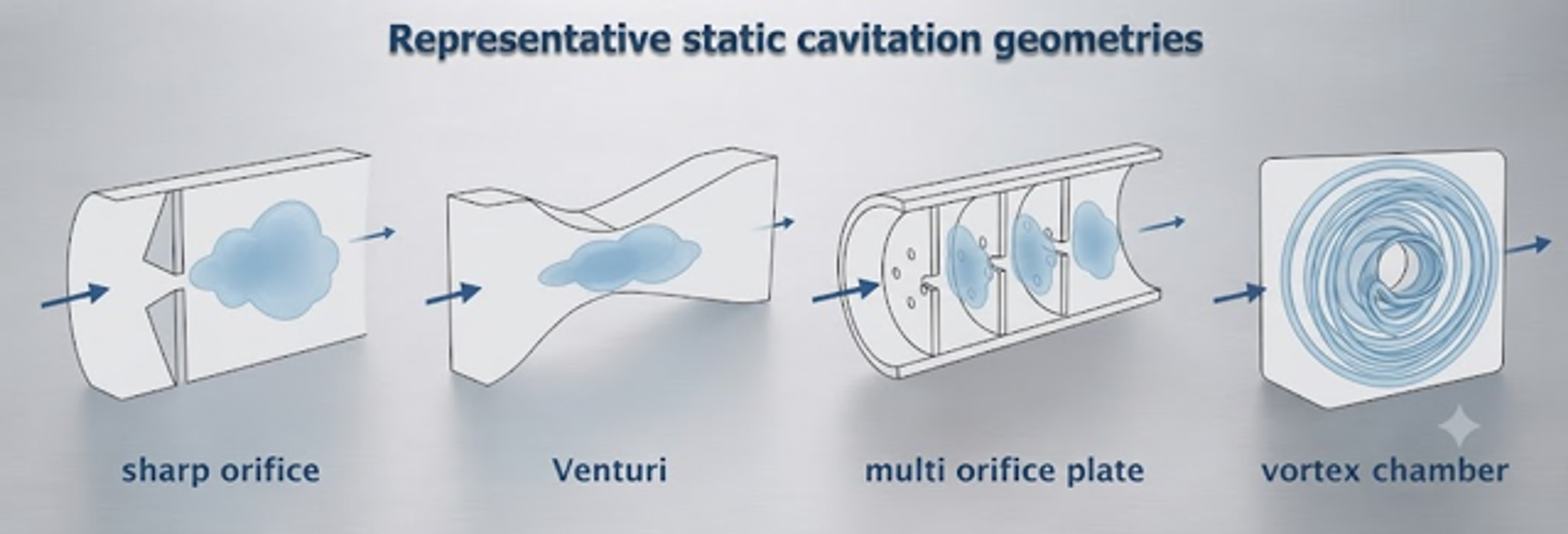
A sharp orifice creates a vena contracta downstream of the plate. Velocity reaches a maximum and static pressure reaches a minimum near this location. Cavities form in low pressure region and collapse as the jet expands. A Venturi provides a more gradual pressure reduction and recovery, often with a lower irreversible pressure loss. Multi orifice plates distribute flow among smaller passages and can increase the number of active cavity zones. Vortex chambers generate low pressure cores through angular momentum rather than a single axial contraction.
Figure 6.2. Representative static hydrodynamic cavitation geometries [58]Source: Kozyuk O. Hydrodynamic Cavitation. Unpublished technical manuscript and supporting data, 2026.
*[Figure 6.2](#figure-6-2). Representative static hydrodynamic cavitation geometries [58].*
The minimum passage dimension must be selected relative to the incoming coarse tail. A passage only slightly larger than is vulnerable to plugging, bridging, and rapid erosion. Staged processing can first remove large agglomerates in a robust passage and then use a finer high intensity stage.
### 6.3 High-pressure nozzles and interaction chambers
High pressure nozzle systems convert pump pressure into a high-velocity jet through passages commonly measured in tens to hundreds of micrometers. Studies of high-pressure homogenization commonly report operation at approximately 100 to 500 bar, with particle size decreasing as pressure and the number of passes increase [14]. Solids may be introduced downstream of the pressure generating pump when exposure of the pump to abrasive material must be minimized. The critical design task is to place the strongest hydrodynamic loading at the contraction and the principal bubble collapse in a downstream chamber where particles are present, but wall erosion remains manageable.
Figure 6.3. High pressure nozzle dispersion loop and qualitative axial profiles of pressure, velocity, vapor fraction, hydrodynamic stress, and collapse-induced stress [58]Source: Kozyuk O. Hydrodynamic Cavitation. Unpublished technical manuscript and supporting data, 2026.
*[Figure 6.3](#figure-6-3). High pressure nozzle dispersion loop and qualitative axial profiles of pressure, velocity, vapor fraction, hydrodynamic stress, and collapse-induced stress [58].*
At sufficiently high fragmentation number, rapid rupture or shattering can dominate over gradual erosion. At lower pressure, higher viscosity, or greater agglomerate strength, more passes may be needed, and the response may become controlled by erosion.
### 6.4 Micro-orifice and cavitation-on-chip systems
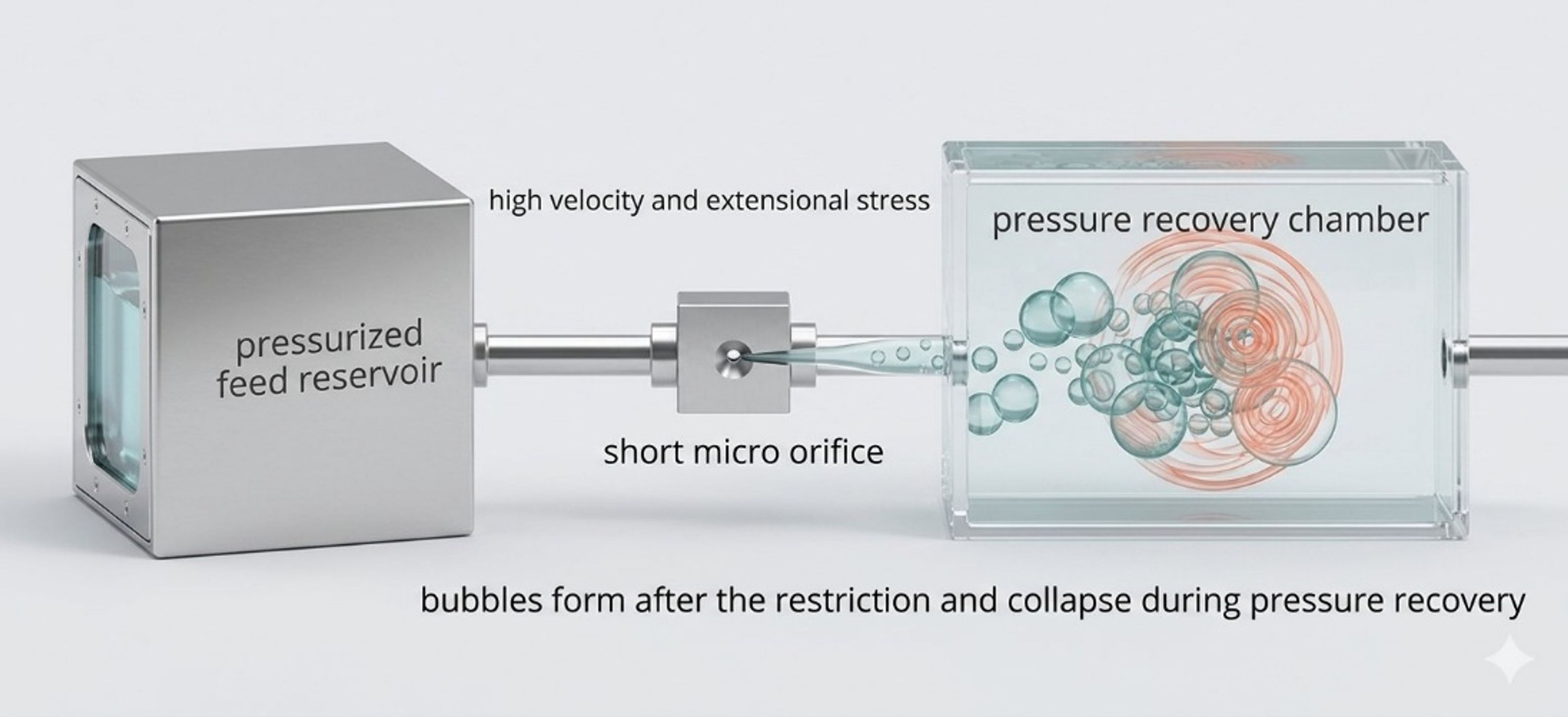
Micro orifice systems direct an agglomerated nanofluid through a short restriction. The passage is selected so that bubbles form near or after the restriction and collapse in a downstream recovery region rather than on the passage wall. Karimzadehkhouei and coworkers used a short channel with a characteristic size near 152 micrometers for alumina nanofluids [23]. Talebian Gevari and coworkers later visualized cavitation and particle breakup in a microfluidic device of similar scale [24].
Figure 6.4. Schematic of a cavitation configuration with a short restriction and downstream collapse region [58]Source: Kozyuk O. Hydrodynamic Cavitation. Unpublished technical manuscript and supporting data, 2026.
*[Figure 6.4](#figure-6-4). Schematic of a cavitation configuration with a short restriction and downstream collapse region [58].*
The related patent describes one or more restrictive elements, optional heating, and series configurations intended to reduce or prevent nanofluid agglomeration [25]. Patent descriptions are useful for equipment architecture but should not be treated as independent validation of performance.
### 6.5 Water jet mills
A water jet mill combines rapid shear, cavitation bubble collapse, direct particle impact, recirculation, and classification [30]. The reported prototype used water pressure near 400 MPa and a nozzle diameter near 0.23 mm. Coarse material was returned to the milling cycle while the fine fraction was separated. Because hard target impact and classification contribute, this device should be described as an integrated cavitation mill rather than a pure deagglomerator. Earlier cavitation studies on ceramic powders also reported nanoscale titania and zirconia products [39].
### 6.6 Jet cavitation devices
Jet and microfluidic cavitation devices have been used to exfoliate graphite and related layered solids [31–33,40]. A typical loop contains a feed or recirculation reservoir, pressure source, micro restriction or cavitation generator, downstream recovery chamber, cooler, and return line. Shear in the contraction acts mainly parallel to the sheets, while pressure recovery and bubble collapse add normal and oblique loading. Repeated exposure can progressively reduce layer count, but excessive cycling can reduce lateral dimension or increase defects.
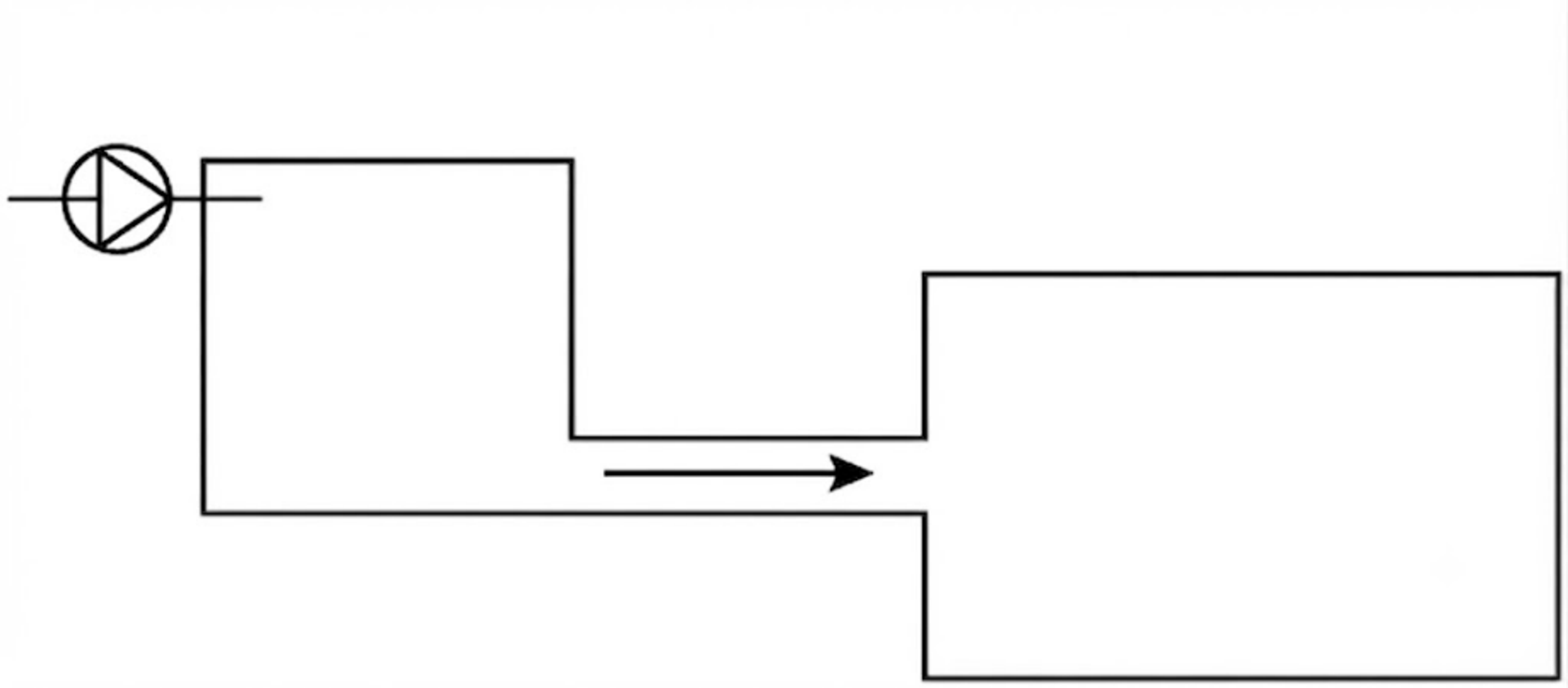
A patent by Ayela and Colombet describes a first small hydraulic diameter section that generates shear and bubbles, followed by a larger section in which bubbles implode and assist exfoliation [34].
Figure 6.5. Two-section flow path for particle exfoliation [34]Source: Ayela F, Colombet D. Method for exfoliating particles. US Patent 11,104,578 B2, 31 August 2021.
*[Figure 6.5](#figure-6-5). Patent drawing of a two-section flow path for particle exfoliation [34].*
The patent specifies a first section hydraulic diameter below 300 micrometers, with preferred values below 150 or 90 micrometers. The design objective is to combine shear and a controlled collapse wave while limiting in-plane fracture [34].
### 6.7 Dynamic cavitation processors and production skids
Dynamic processors use rotating disks, perforations, teeth, grooves, blades, or rotor stator gaps to create repeated low pressure zones and recovery regions. Compared with static restrictions, they can process higher flow at lower external pressure and may tolerate more viscous formulations. Their performance is governed by tip speed, gap size, stage count, rotor geometry, gas management, and recirculation. Mechanical power includes useful liquid work and parasitic losses in bearings, seals, and bulk circulation.
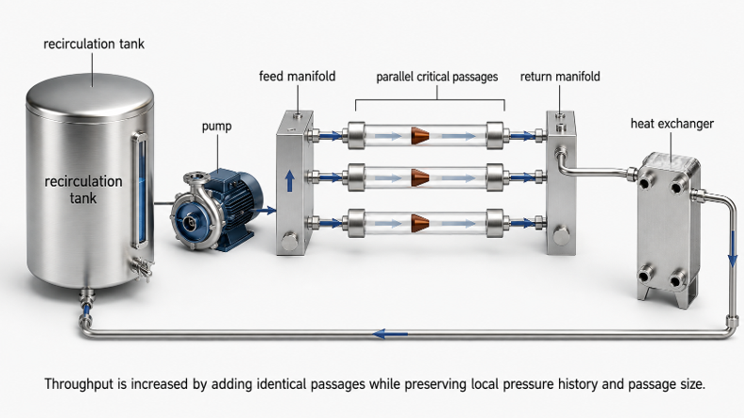
A production skid normally includes a feed or recirculation tank, pump, pressure control, heat exchanger, cavitation reactor, sampling ports, relief devices, and optional filtration or classification. Abrasive solids require replaceable wear inserts, pressure-resistant bypass lines, and a monitoring plan for elemental contamination. Cleaning design becomes critical when the allowable top size approaches the smallest flow passage.
## 7 Characterization and interpretation
### 7.1 Particle size methods
No single analytical method proves deagglomeration. Laser diffraction is robust over a broad size range and is well suited to micron-scale distributions, but the result depends on refractive index, absorption, obscuration, and dispersion procedure. Dynamic light scattering is useful for dilute nanofluids but is strongly weighted toward large scatterers and may conceal small populations when a coarse tail is present. Sedimentation methods depend on density and shape assumptions. Image analysis can measure shape and agglomeration directly but requires statistically representative sampling.
*Table 7.1. Recommended characterization methods.*
| **Method** | **Main output** | **Strength** | **Important limitation** |
|---------------------------|------------------------------------------------------------|------------------------------------------------------|--------------------------------------------------------|
| Laser diffraction | Volume based equivalent diameter distribution | Wide dynamic range and good process comparison | Optical model and dilution can change result |
| Dynamic light scattering | Intensity, volume, or number transformed hydrodynamic size | Sensitive to nanometer scale agglomeration | Strong bias toward large scatterers and dilute samples |
| SEM | Surface morphology and cluster structure | Direct visual evidence of agglomeration and fracture | Drying may create artifacts |
| TEM | Primary particles, aggregates, layers, defects | High spatial resolution | Small field and demanding preparation |
| AFM | Platelet thickness and surface topology | Useful for exfoliated sheets | Substrate deposition bias |
| X ray diffraction | Crystal phase and coherent domain size | Detects phase change and crystallite order | Does not measure wet agglomerate size |
| Raman spectroscopy | Bonding, defects, layer response | Important for carbon and layered materials | Local heating and fluorescence |
| Rheometry | Viscosity, yield stress, thixotropy | Captures network structure at process concentration | Sensitive to shear history and temperature |
| Zeta potential | Electrokinetic potential | Useful formulation screen | Not a universal stability criterion |
| ICP or elemental analysis | Dissolved and particulate metals | Detects equipment wear | Requires representative digestion and blanks |
### 7.2 Sampling and method control
A defensible test protocol should specify feed preparation, mixing time, temperature, solids content, sampling location, analytical dilution, dispersant, analytical sonication, optical properties, and the elapsed time between processing and measurement. Analytical sonication can erase the distinction between process performance and sample preparation. If sonication is used, control and processed samples must receive the same defined treatment.
Defined analytical preparation is especially important for nanostructured powders. Retamal Marín and coworkers showed that the measured size response to a fixed dispersing energy depends strongly on silica morphology, and that excessive probe energy can introduce metallic wear particles into the sample [57]. Although that study used ultrasonic preparation, the measurement lesson is directly applicable here: the analytical method must not create more breakage or contamination than the process being evaluated. A particle-size report should therefore state the preparation energy, duration, vessel geometry, temperature, and blank contamination result.
At least five response groups are recommended:
- Immediate particle-size distribution and coarse particle count.
- Aged particle size after a defined storage period and temperature cycle.
- Microscopy that distinguishes cluster separation from primary particle fracture.
- Rheology at the final solids concentration.
- Purity, crystal structure, coating integrity, or functional performance as required by the product.
### 7.3 Interpreting a reduction in instrument size
A final DLS diameter of 250 nm does not imply that primary particles were fractured to 250 nm. It means that the hydrodynamic scattering objects have that effective size under the measurement conditions. Similarly, a reduction in laser diffraction may result from cluster separation, erosion, fracture, a refractive index change, or a change in entrained gas. Microscopy and structure sensitive methods are needed to identify the mechanism.
## 8 Material case studies
### 8.1 Zinc oxide
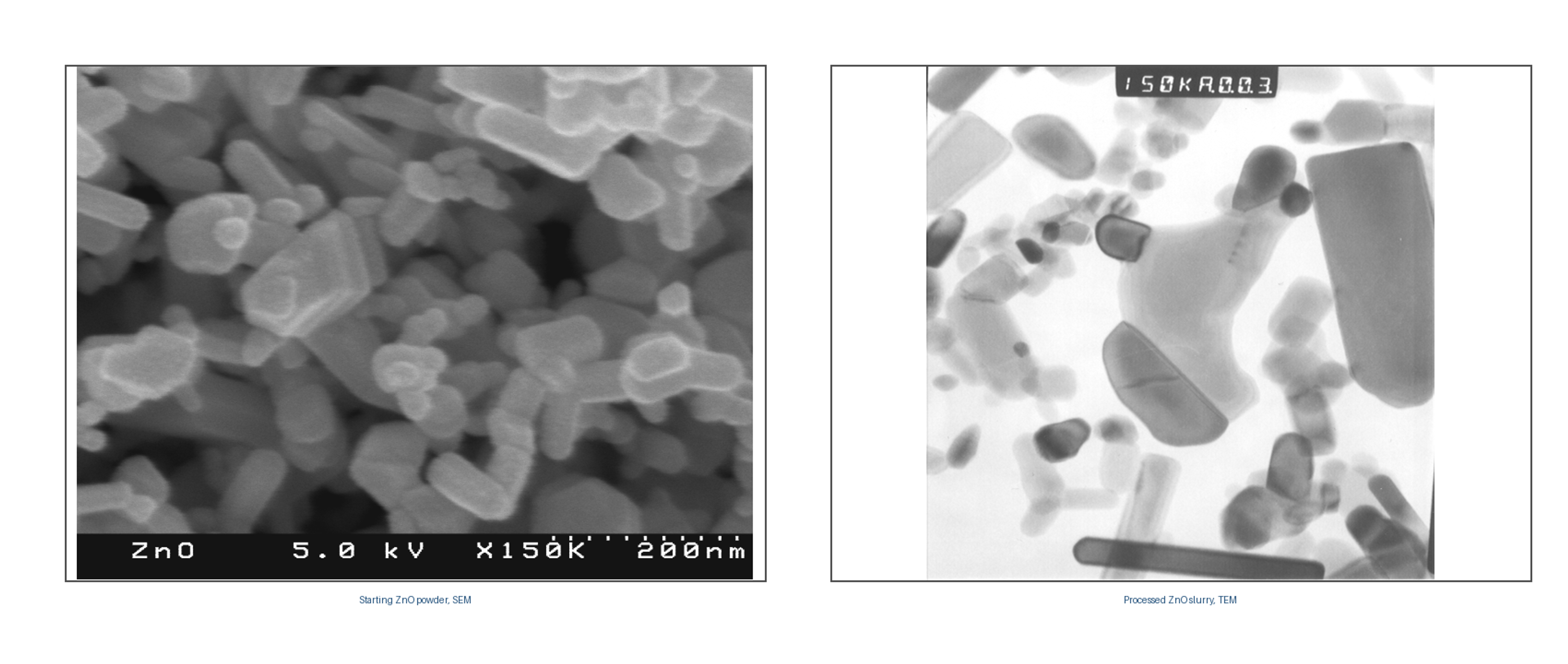
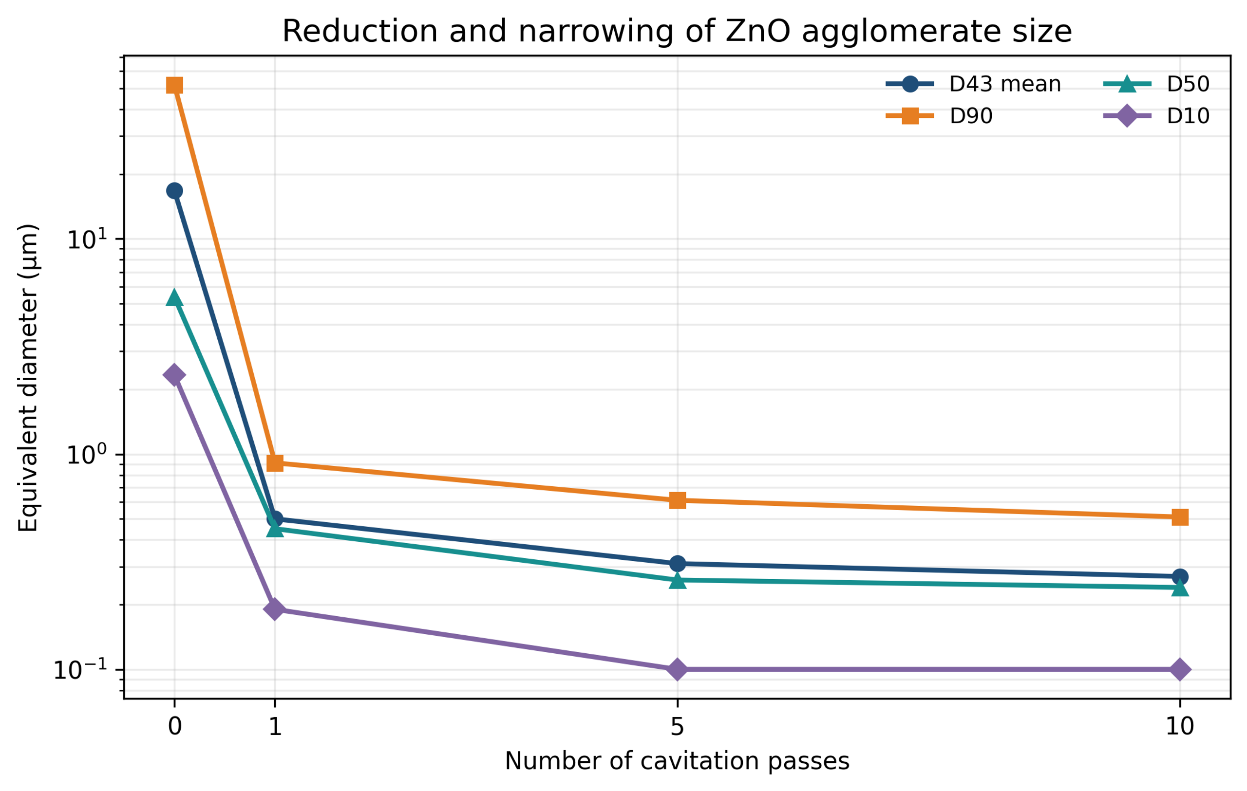
The supplied results describe cavitation-assisted dispersion of a commercial ZnO powder with an average crystallite size of approximately 67 nm and micron sized agglomerates [1,2]. The volume-weighted mean diameter decreased from 16.73 µm in the control sample to 0.50 µm after one pass, 0.31 µm after five passes, and 0.27 µm after ten passes. The D90 value decreased from 51.93 to 0.91 µm after one pass and to 0.51 µm after ten passes.
Figure 8.1. Starting ZnO powder observed by SEM and processed ZnO observed by TEM [2]Source: Kozyuk OV. Particle size reduction and deagglomeration. Technical manuscript and supporting data, undated.
*[Figure 8.1](#figure-8-1). Starting ZnO powder observed by SEM and processed ZnO observed by TEM [2].*
Figure 8.2. Reduction and narrowing of ZnO agglomerate size with cavitation passes [1,2]Sources: Michel FC Jr, Kozyuk O. Hydrodynamic cavitation processing, 2015; Kozyuk OV. Particle size reduction and deagglomeration, undated.
*[Figure 8.2](#figure-8-2). Reduction and narrowing of ZnO agglomerate size with cavitation passes [1,2].*
*Table 8.1. ZnO particle size response to number of passes.*
| **Passes** | mean (µm) | (µm) | (µm) | (µm) |
|------------|-------------------------------|-------------------------|-------------------------|-------------------------|
| Control | 16.73 | 51.93 | 5.37 | 2.33 |
| 1 | 0.50 | 0.91 | 0.45 | 0.19 |
| 5 | 0.31 | 0.61 | 0.26 | 0.10 |
| 10 | 0.27 | 0.51 | 0.24 | 0.10 |
The large improvement after the first pass, followed by smaller incremental changes, is consistent with a broad strength distribution. Weak agglomerates fail early, whereas the remaining structures have stronger contacts or approach an endpoint limited by stabilization. The 0.27 micrometer mean should not be interpreted as crystallite size. The evidence is predominantly consistent with deagglomeration, although some aggregate erosion cannot be excluded.
### 8.2 Bentonite clay
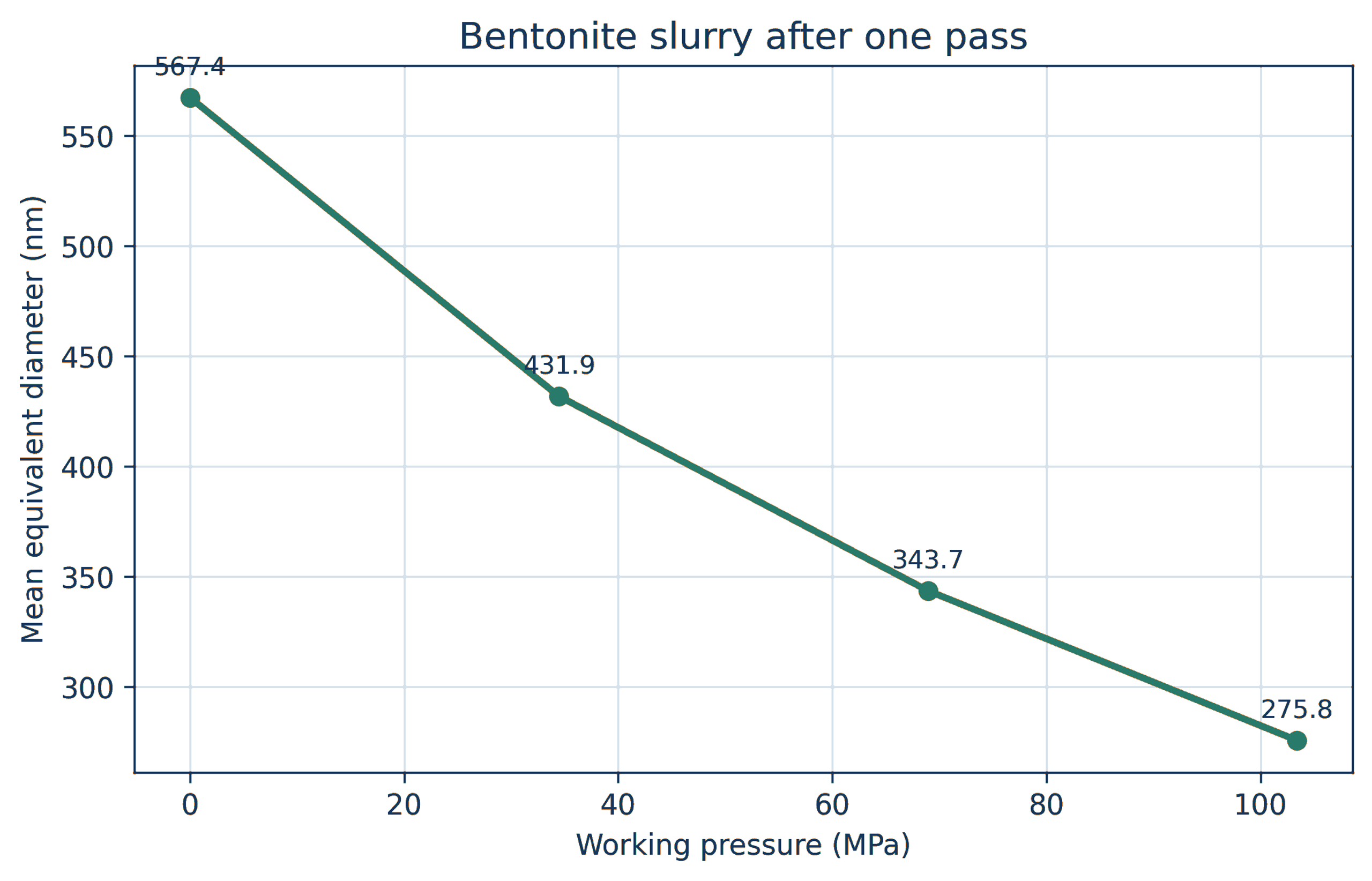
A 5 wt% bentonite slurry showed a pressure-dependent decrease in mean equivalent diameter after one pass. The mean decreased from 567.4 nm in the control to 431.9 nm at 34.47 MPa, 343.7 nm at 68.95 MPa, and 275.8 nm at 103.42 MPa [1,2].
Figure 8.3. Mean diameter of a 5 wt% bentonite slurry after one pass at increasing pressure [1,2]Sources: Michel FC Jr, Kozyuk O. Hydrodynamic cavitation processing, 2015; Kozyuk OV. Particle size reduction and deagglomeration, undated.
*[Figure 8.3](#figure-8-3). Mean diameter of a 5 wt% bentonite slurry after one pass at increasing pressure [1,2].*
Bentonite response depends strongly on hydration time, exchangeable cation, ionic strength, pH, and platelet chemistry. A pressure response measured in one aqueous formulation cannot be transferred directly to another. Rheology may change more strongly than median size because a small amount of delaminated high aspect ratio material can alter the network.
### 8.3 Silver powder and nanosilver dispersions
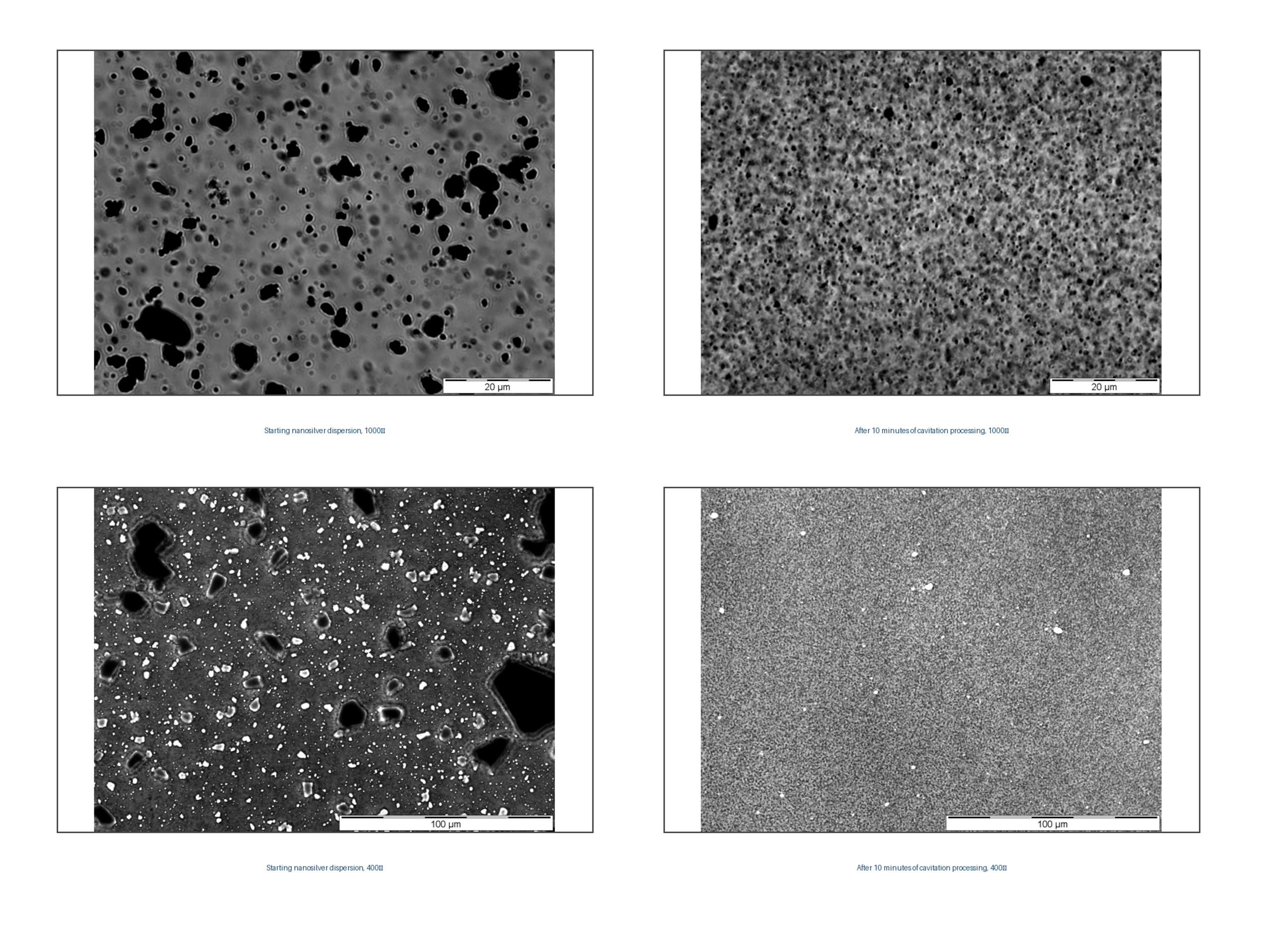
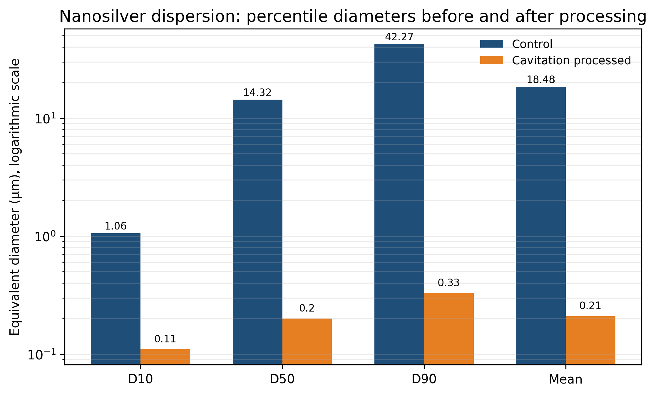
Silver powders for conductive inks often contain nanoscale or submicron primary particles assembled into clusters tens of micrometers in size. The supplied nanosilver data show a control with micrometers, micrometers, micrometers, and a mean of 18.48 micrometers. After 10 minutes of controlled flow cavitation processing, the corresponding values were 0.11, 0.20, 0.33, and 0.21 micrometers [2,26].
Figure 8.4. Nanosilver dispersion before and after 10 minutes of cavitation processing at 1000× and 400× magnification [2,26]Sources: Kozyuk OV. Particle size reduction and deagglomeration, undated; Five Star Technologies. Custom Silver Dispersions, undated.
*[Figure 8.4](#figure-8-4). Nanosilver dispersion before and after 10 minutes of cavitation processing at 1000× and 400× magnification [2,26].*
Figure 8.5. Percentile diameters of nanosilver before and after cavitation processing [2,26]Sources: Kozyuk OV. Particle size reduction and deagglomeration, undated; Five Star Technologies. Custom Silver Dispersions, undated.
*[Figure 8.5](#figure-8-5). Percentile diameters of nanosilver before and after cavitation processing [2,26].*
*Table 8.2. Nanosilver particle size distribution.*
| **Condition** | **(µm)** | **(µm)** | **(µm)** | **Mean (µm)** |
|----------------------|-------------------------------------|-------------------------------------|-------------------------------------|---------------|
| Control | 1.06 | 14.32 | 42.27 | 18.48 |
| Cavitation processed | 0.11 | 0.20 | 0.33 | 0.21 |
The result demonstrates strong elimination of the coarse tail. For conductive flakes, however, excessive fracture can reduce aspect ratio and alter percolation, packing, viscosity, and cured conductivity. The correct target may be separation of flake clusters rather than grinding of each flake. Microscopy and electrical testing are therefore required in addition to particle-size measurement.
### 8.4 Silica, silver flakes, and carbon nanofibers in resin
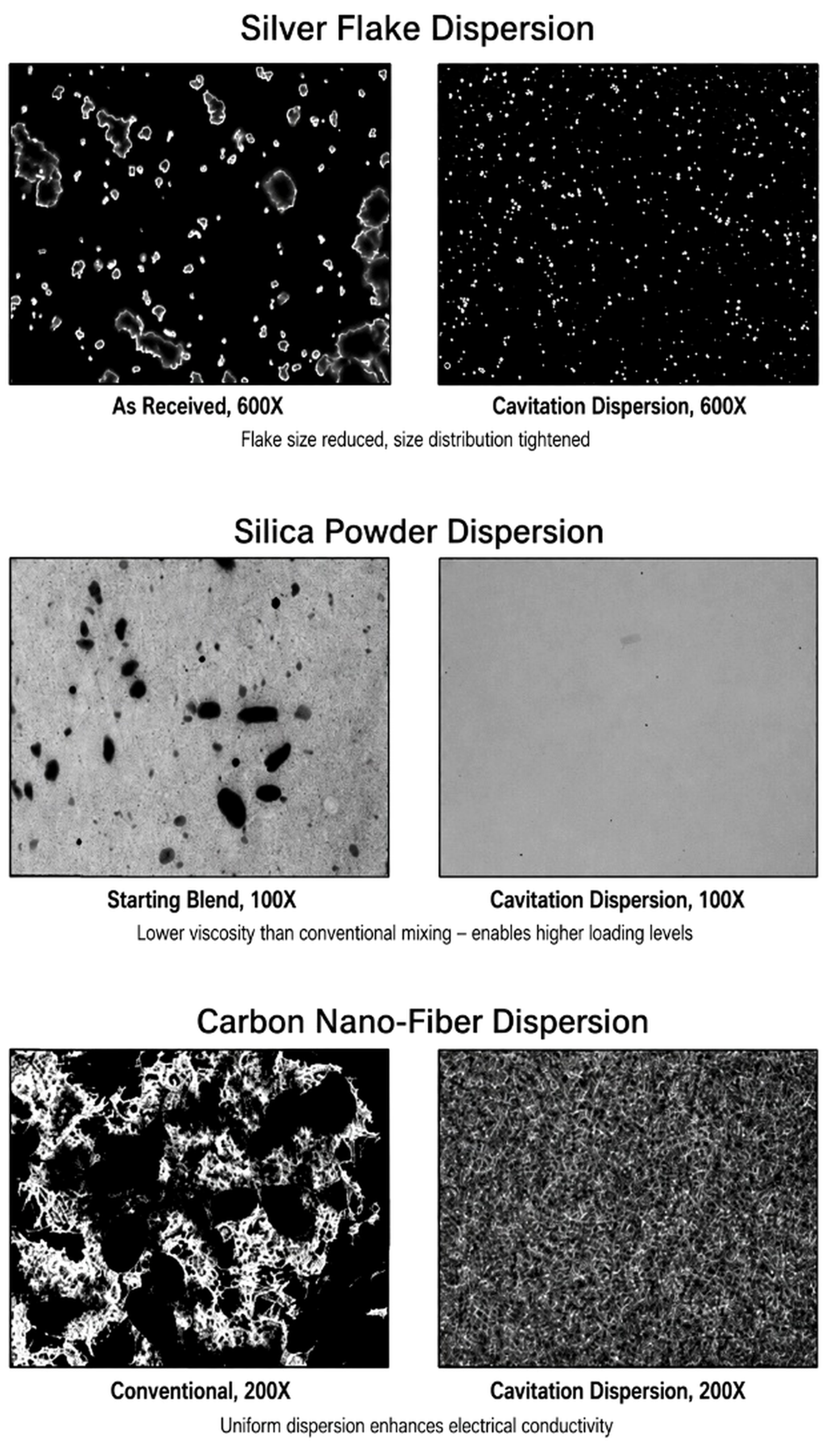
[Figure 8.6](#figure-8-6) presents before and after micrographs of silver flakes, silica powder, and carbon nanofibers in resin media [27,28]. Data from these materials indicate a denser flake distribution, lower viscosity in silica filled systems, and a more uniform carbon nanofiber network with improved conductivity. These examples demonstrate the range of compositions that can be processed.
Figure 8.6. Before and after micrographs of silver flake, silica powder, and carbon nanofiber dispersions [27,28]Sources: Five Star Technologies. Dispersion Services, 2009; Five Star Electronic Dispersions Overview, undated.
*[Figure 8.6](#figure-8-6). Before and after micrographs of silver flake, silica powder, and carbon nanofiber dispersions [27,28].*
In filled resins, effectiveness is limited by viscosity and the ability to drive the formulation through small passages. Processing may be performed in a lower viscosity carrier followed by letdown, or in a heated resin within its stability window. Polymer chain scission, gas entrainment, and local overheating should be evaluated.
### 8.5 Soy slurry particle size reduction
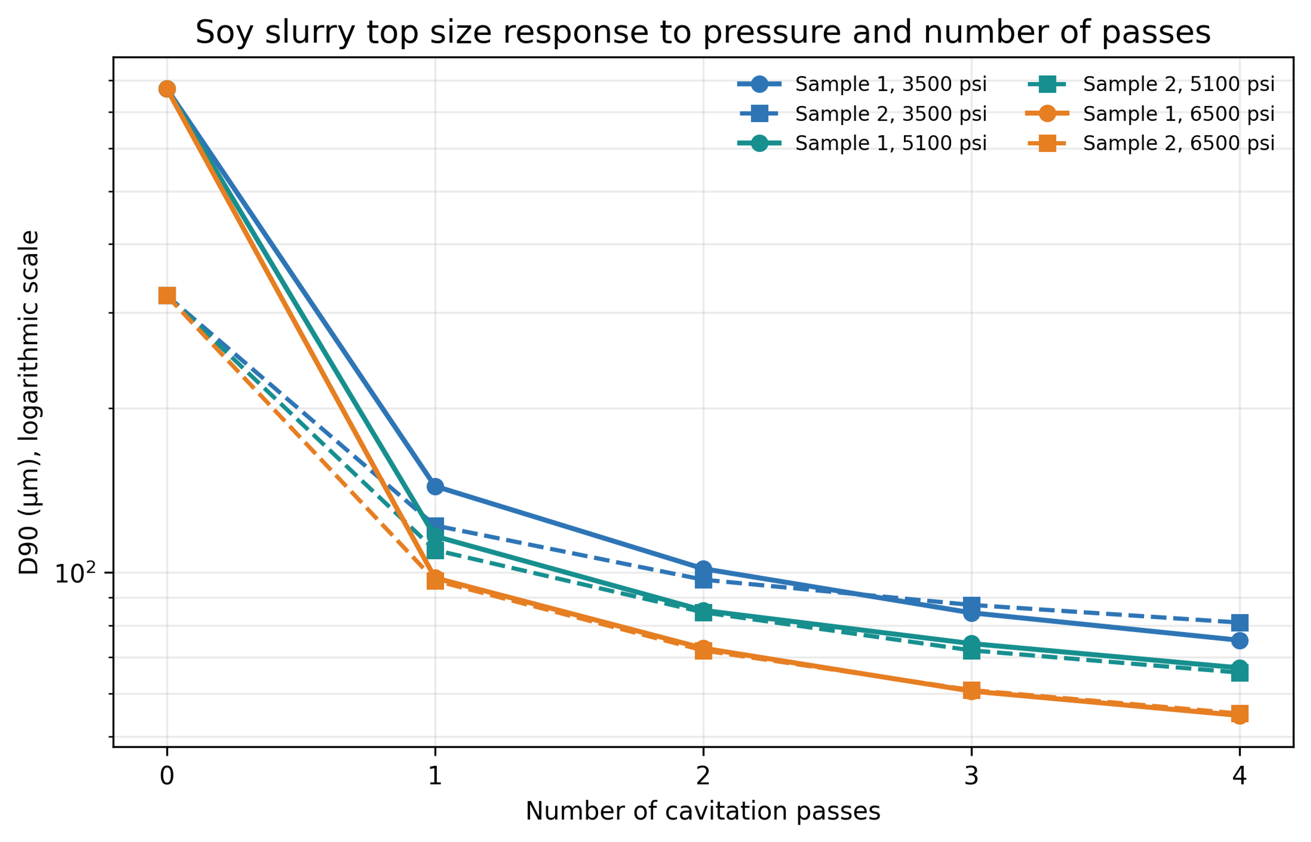
In studies conducted by Arisdyne Systems, two variants of the initial soybean slurry were evaluated at pressures of 3,500, 5,100, and 6,500 psi and with one to four passes [29]. The samples were heated to approximately 70 to 75 °C, and their characteristics were measured five times using a Horiba LA950 analyzer. Sample 1 consisted of a previously ground slurry with a coarser particle size, whereas Sample 2 had undergone additional grinding.
Figure 8.7. Soy slurry response to pressure and number of passes [29]Source: Arisdyne Systems. Processing of Soy Slurry to Reduce Particle Size, November 2018.
*[Figure 8.7](#figure-8-7). Soy slurry response to pressure and number of passes [29].*
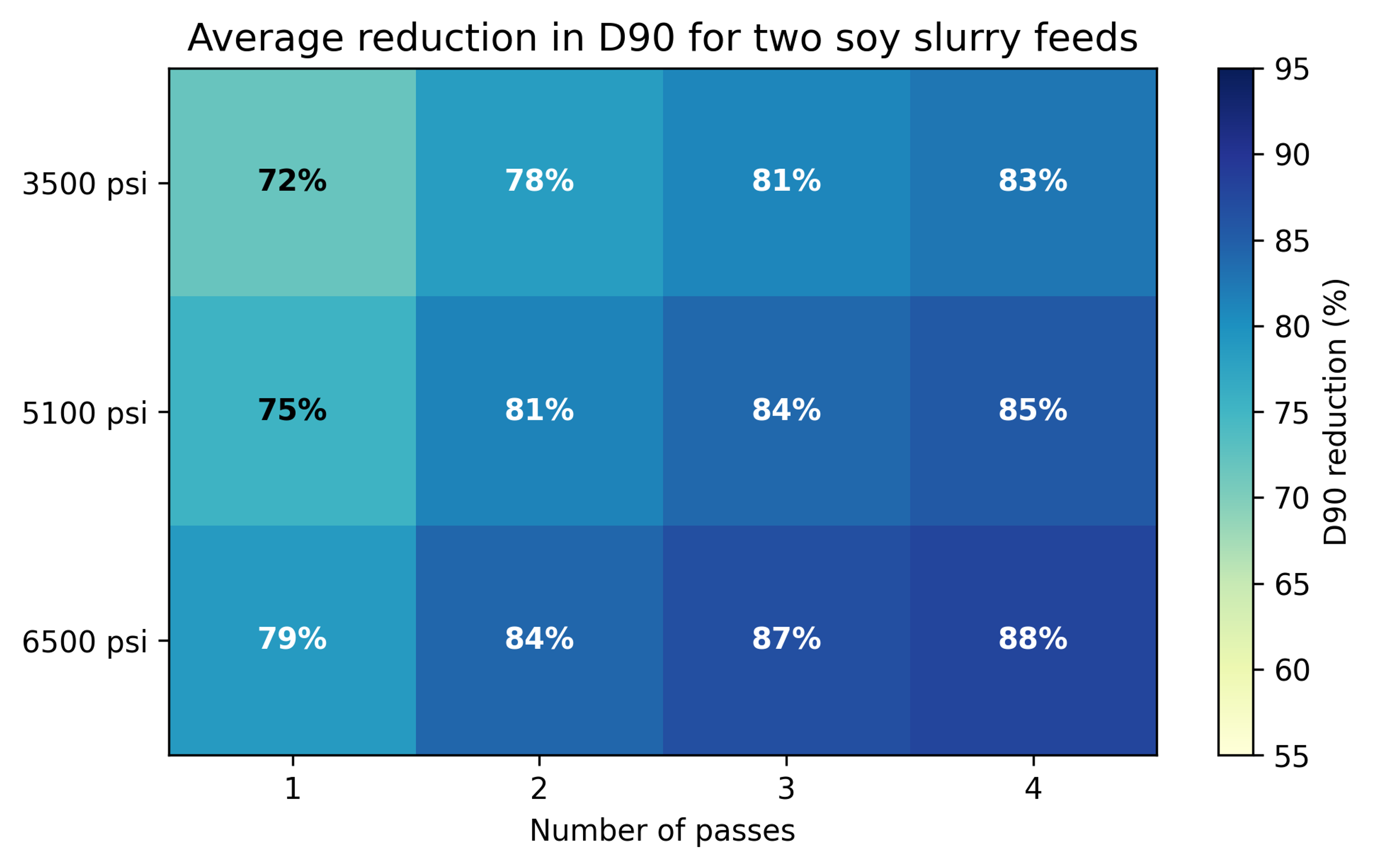
Figure 8.8. Average percent reduction in for two soy slurry feeds. Calculation from supplied data [29]Source: Arisdyne Systems. Processing of Soy Slurry to Reduce Particle Size, November 2018.
*[Figure 8.8](#figure-8-8). Average percent reduction in for two soy slurry feeds. Calculation from supplied data [29].*
*Table 8.3. Selected soy slurry and values.*
| **Feed and condition** | **(µm)** | **(µm)** |
|------------------------------|-------------------------------------|-------------------------------------|
| Sample 1 control | 182.304 | 772.039 |
| Sample 1, 3500 psi, 1 pass | 64.448 | 144.019 |
| Sample 1, 5100 psi, 2 passes | 45.075 | 85.230 |
| Sample 1, 6500 psi, 4 passes | 27.043 | 54.690 |
| Sample 2 control | 127.352 | 322.033 |
| Sample 2, 3500 psi, 1 pass | 61.350 | 121.976 |
| Sample 2, 5100 psi, 2 passes | 44.098 | 84.549 |
| Sample 2, 6500 psi, 4 passes | 27.104 | 55.130 |
Both feeds approached a similar endpoint near micrometers and micrometers at 6,500 psi after four passes. Higher pressure reduced the number of passes required for a comparable result. The distributions also became narrower and less bimodal. Because the samples had been frozen for shipment, the report notes that freeze and thaw history may have affected cell wall damage and control particle size [29].
### 8.6 Alumina and titania nanofluids
Karimzadehkhouei and coworkers used a short micro orifice to process heated gamma alumina nanofluids [23]. In one test series, the mean hydrodynamic diameter decreased from approximately 1718 nm after heating to 1281 nm at 10 bar and 825 nm at 60 bar. In the second series, values of 515 nm at 60 bar and 255 nm at 90 bar were reported. Lower cavitation number correlated with greater deagglomeration.
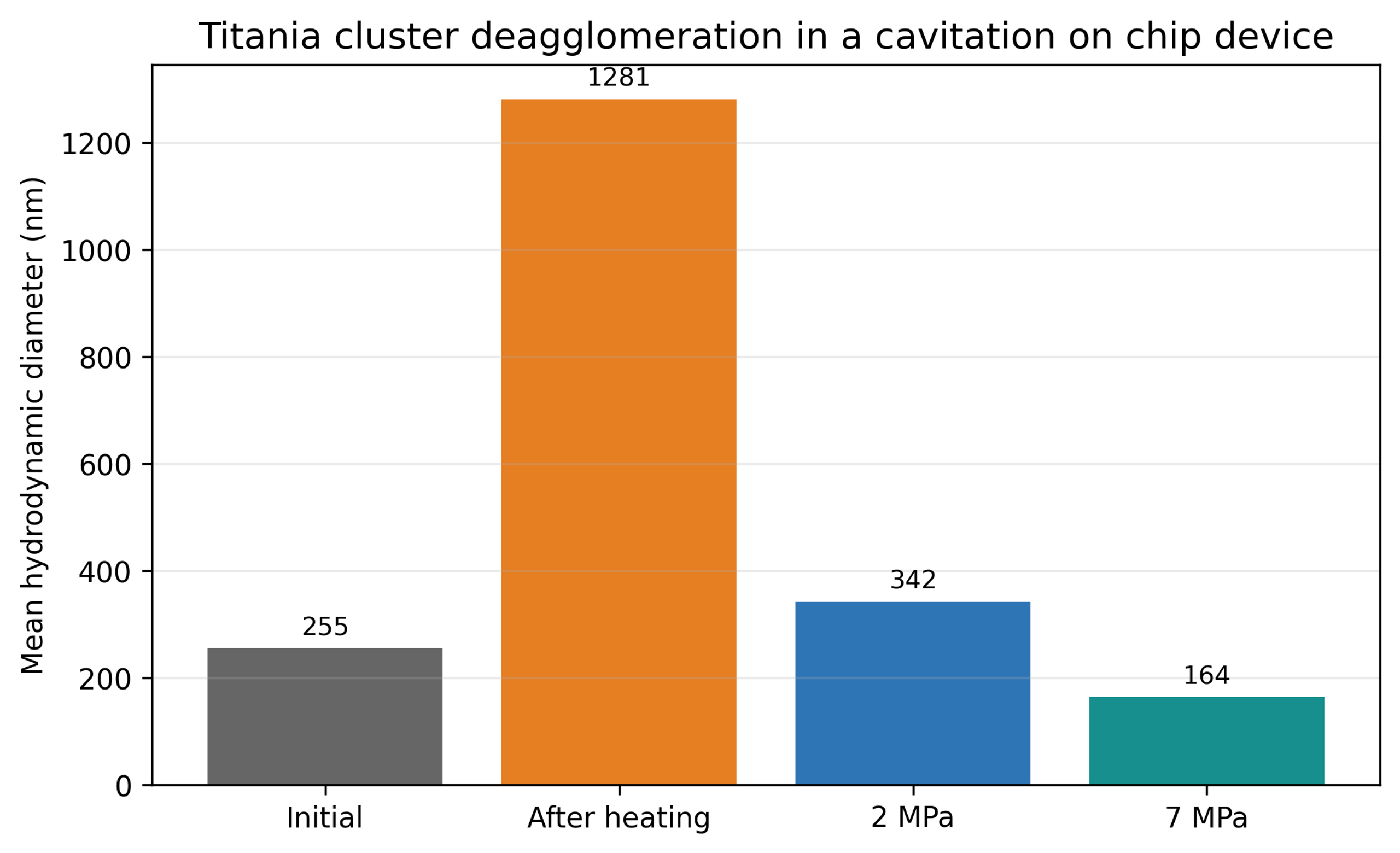
A later cavitation on chip study used dilute titania nanofluid and direct high-speed visualization [24]. The mean hydrodynamic diameter increased from 255 nm to 1281 nm after thermal agglomeration, then decreased to 342 nm at 2 MPa and 164 nm at 7 MPa.
Figure 8.9. Titania cluster deagglomeration in a cavitation on chip device [24]Source: Talebian Gevari M et al. Deagglomeration of nanoparticle clusters in a cavitation on chip device. AIP Advances, 2020.
*[Figure 8.9](#figure-8-9). Titania cluster deagglomeration in a cavitation on chip device [24].*
The authors estimated local impact pressure scales of approximately 80 to 175 MPa for the modeled conditions [24]. These are local model-based estimates, not uniform stresses measured throughout the device. The final DLS size represents hydrodynamic agglomerates and does not indicate fracture to the same primary particle size.
### 8.7 Silicon nanomilling
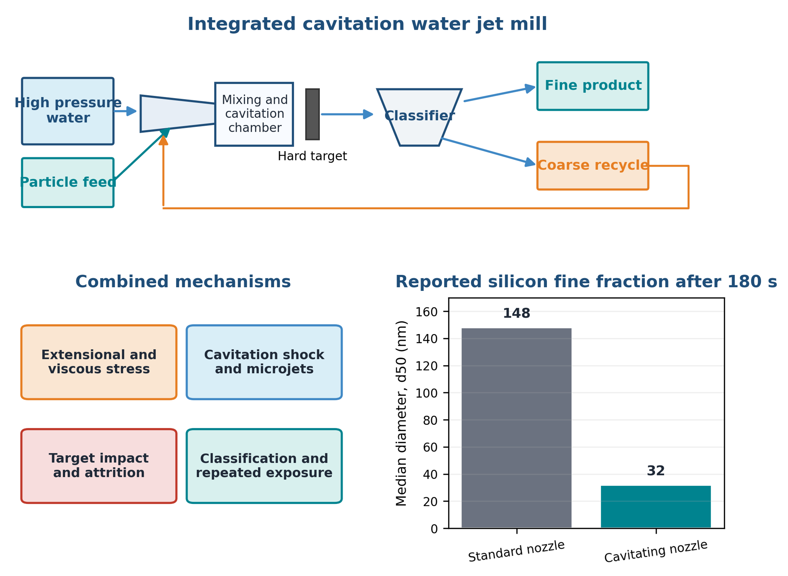
The water jet mill study began with monocrystalline silicon particles with a maximum size near 100 micrometers [30]. After 180 seconds, a standard high-pressure nozzle produced a separated fine fraction with a median near 148 nm. A cavitating nozzle produced a reported median near 32 nm under otherwise comparable conditions.
Figure 8.10. Integrated water jet mill loop, active mechanisms, and reported silicon median size after 180 seconds [30]Source: Dvorský R et al. Preparation of silicon nanoparticles by means of disintegration in a cavitation water jet. NANOCON 2010.
*[Figure 8.10](#figure-8-10). Integrated water jet mill loop, active mechanisms, and reported silicon median size after 180 seconds [30].*
This case combines deagglomeration and comminution with target impact, recirculation, and classification. It should not be used as evidence that cavitation alone produced the complete size reduction. Energy allocation among jet kinetic energy, heating, cavitation, impact, and classification is also difficult.
### 8.8 Exfoliation of graphite and production of few layer graphene
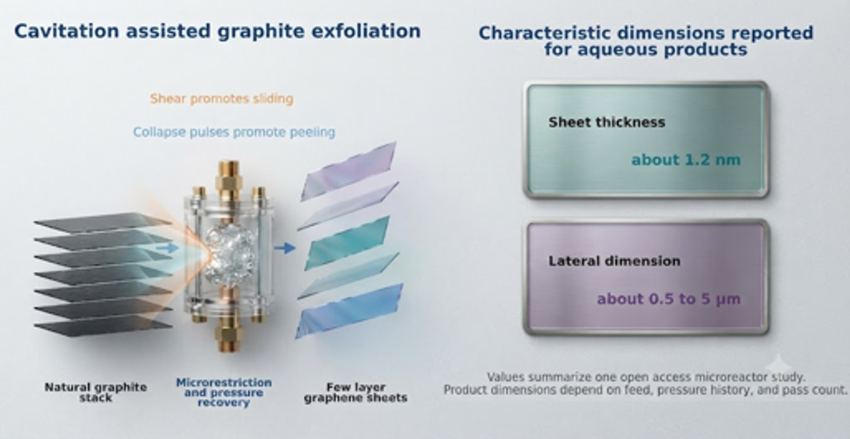
Layered materials have strong in-plane bonding and weaker interlayer attraction. In hydrocavitating microchannels, acceleration and wall shear can initiate sliding or peeling, while pressure recovery, microjets, and collapse waves act normal or oblique to the sheets. Open access studies of natural graphite demonstrate that these effects can be combined in water-based microreactors and recirculating flow paths [31,33,40].
Figure 8.11. Cavitation assisted graphite exfoliation mechanism and reported characteristic dimensions of aqueous few-layer graphene products [58]Source: Kozyuk O. Hydrodynamic Cavitation. Unpublished technical manuscript and supporting data, 2026.
*[Figure 8.11](#figure-8-11). Cavitation assisted graphite exfoliation mechanism and reported characteristic dimensions of aqueous few-layer graphene products [58].*
Qiu and coworkers used a hydrocavitating lab on a chip to exfoliate natural graphite in an aqueous surfactant suspension and reported monolayer and few-layer graphene with lateral dimensions around 300 nm [31]. Jafarpour and coworkers later described aqueous exfoliation of natural graphite in a microfluidic cavitation reactor without surfactant and reported sheets with thickness near 1.2 nm and lateral dimensions from approximately 0.5 to 5 micrometers [33]. The desired product is a thin sheet with preserved lateral size and low defect density. Overprocessing can reduce lateral size or introduce defects, so thickness, lateral dimension, Raman response, diffraction, and defect density should be measured together.
### 8.9 Pharmaceutical wet milling and crystallization
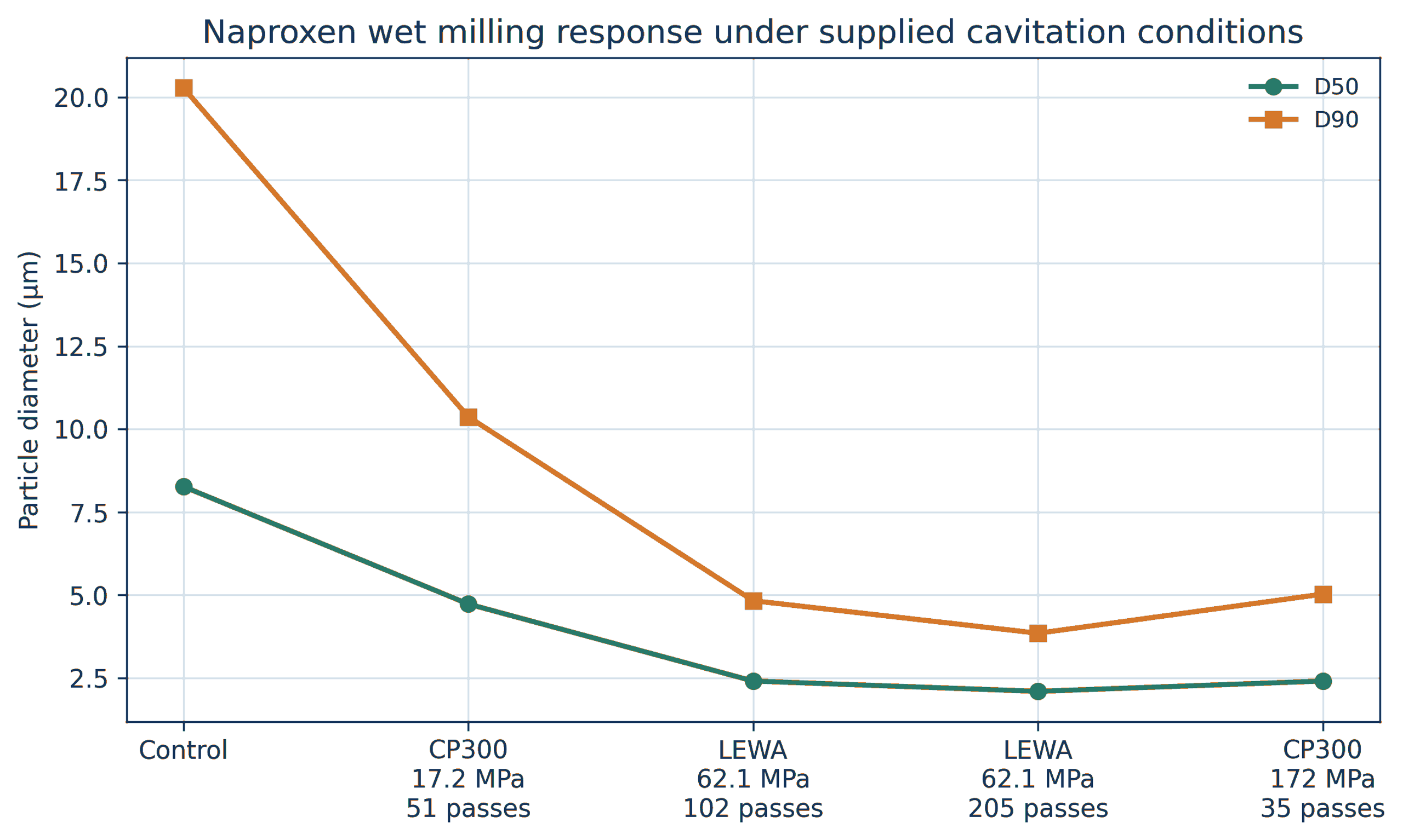
The supplied data compare cavitation processing conditions for naproxen in water containing hydroxypropyl cellulose and sodium lauryl sulfate [1]. The control had micrometers and micrometers. A CP300 condition at 2,500 psi and approximately 50.7 cumulative passes produced micrometers and micrometers. A LEWA condition at 9,000 psi and approximately 204.7 passes produced micrometers and micrometers.
Figure 8.12. Naproxen median and upper tail particle sizes under supplied wet milling conditions [1]Source: Michel FC Jr, Kozyuk O. Hydrodynamic cavitation processing. Royal Society of Chemistry, 2015.
*[Figure 8.12](#figure-8-12). Naproxen median and upper tail particle sizes under supplied wet milling conditions [1].*
Pressure alone did not determine performance. The 9,000 psi LEWA condition with greater cumulative exposure produced a smaller upper tail than the 25,000 psi CP300 condition with fewer passes. Geometry, local stress, pass distribution, and cumulative exposure must be considered together.
Tiwari and coworkers compared hydrodynamic cavitation, ultrasound, and wet milling for paracetamol particle engineering in saturated solution [36]. Their vortex cavitation device produced a larger fine fraction than the comparison methods under the tested conditions and demonstrated that cavitation can be integrated with crystallization rather than used only as a post milling step. Pharmaceutical development must verify polymorphic form, chemical stability, dissolution, excipient integrity, sterility strategy, and metal contamination. General pharmaceutical nanomilling practice also emphasizes stabilizer selection, temperature control, process energy, and verification of solid state form [17].
### 8.10 Cavitation induced agglomeration in CMP slurries
Cavitation does not always disperse particles. Litchy and coworkers circulated fumed silica, colloidal silica, alumina, and ceria chemical mechanical planarization slurries through several pump types [37]. When inlet pressure was reduced while nominal shear remained similar, some formulations developed a larger coarse particle population. The effect was especially pronounced for fumed silica and depended strongly on formulation.
Possible mechanisms include collapse-induced compaction, damage to stabilizing surface layers, gas-liquid interface effects, local concentration gradients, intense collisions, and rapid reattachment of fresh surfaces. The practical lesson is that higher cavitation intensity is not automatically better. Every formulation has a process window.
*Table 8.4. Summary of selected quantitative case studies.*
| **Material** | **Starting condition** | **Reported cavitation result** | **Dominant interpretation** | **Source** |
|--------------------------|----------------------------------|---------------------------------------------------------------------------------------------------------------------|-----------------------------------------------|------------|
| ZnO | Mean agglomerate size 16.73 µm | 0.50 µm after one pass and 0.27 µm after ten passes | Predominantly deagglomeration | [1,2] |
| Bentonite, 5 wt% | Mean 567.4 nm | 275.8 nm after one pass at 103.42 MPa | Tactoids and cluster disruption | [1,2] |
| Nanosilver | µm | µm | Strong coarse tail elimination | [2,26] |
| Soy slurry, coarse feed | µm | µm at 6500 psi and four passes | Cell and particle disruption plus narrowing | [29] |
| Heated titania nanofluid | Mean 1281 nm | 164 nm at 7 MPa | Deagglomeration | [24] |
| Silicon | Feed maximum near 100 µm | Cavitating nozzle output median 32 nm | Cavitation, shear, impact, and classification | [30] |
| Graphite | Natural graphite flakes in water | Few layer graphene nanosheets; sheet thickness near 1.2 nm and lateral size about 0.5 to 5 micrometers in one study | Exfoliation with thickness reduction | [31,33] |
| CMP fumed silica | Stabilized polishing slurry | Coarse particle population increased | Cavitation assisted agglomeration | [37] |
### 8.11 Iron oxide in water and mixed solvent media
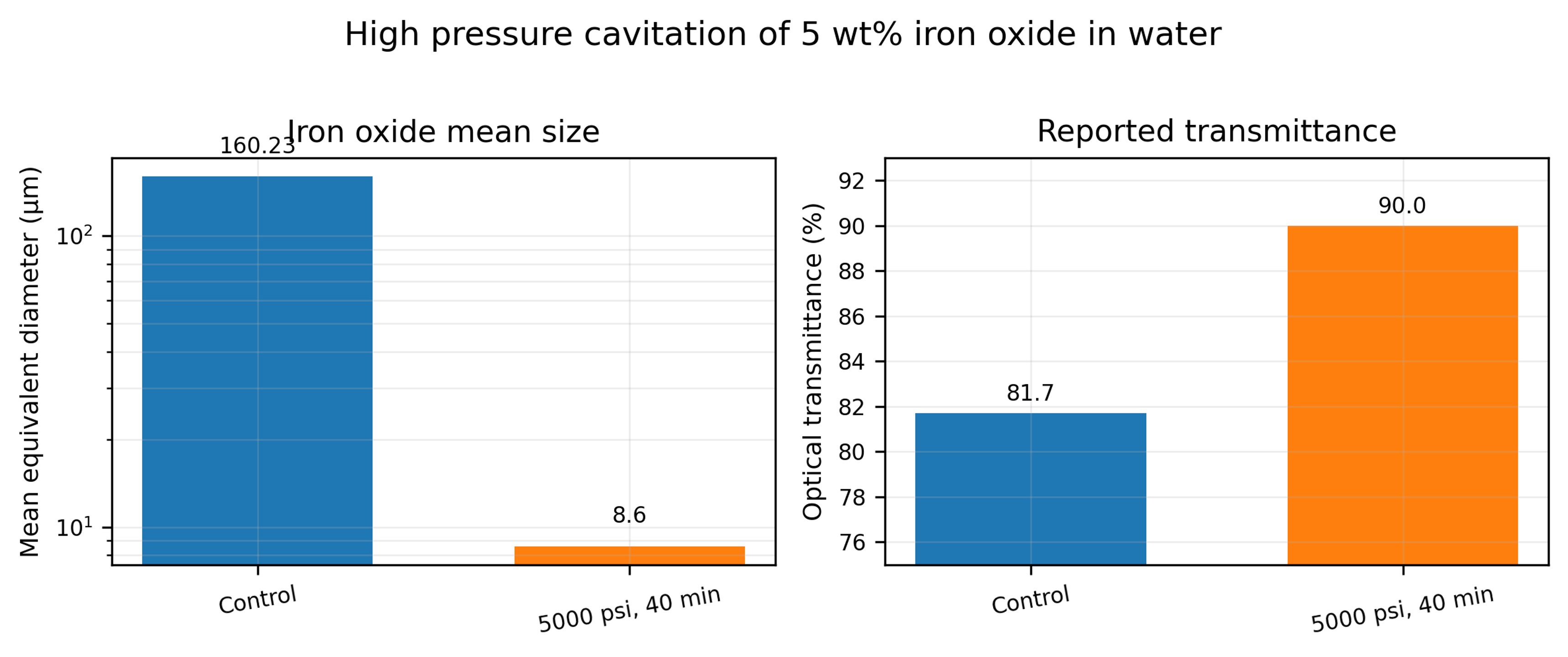
An internal test processed a 5 wt% iron oxide suspension in distilled water through a CP300 system fitted with elements 12 and 14. The feed hopper was agitated at 800 rpm, the operating pressure was 5,000 psi (34.47 MPa), the bulk temperature was held at 25 °C, and the material was recirculated for 40 minutes, corresponding to slightly more than 16 nominal passes. The reported mean equivalent diameter decreased from 160.23 µm to 8.6 µm, while optical transmittance increased from 81.7 to 90.0 percent [48]. The diameter reduction was 94.6 percent. Because no microscopy or crystallite measurement was reported, the data establish a reduction in suspended object size but do not distinguish weak agglomerate separation from aggregate or crystal fracture.
For comparison among different feeds, a useful descriptive quantity is the deagglomeration factor:
(8.1)
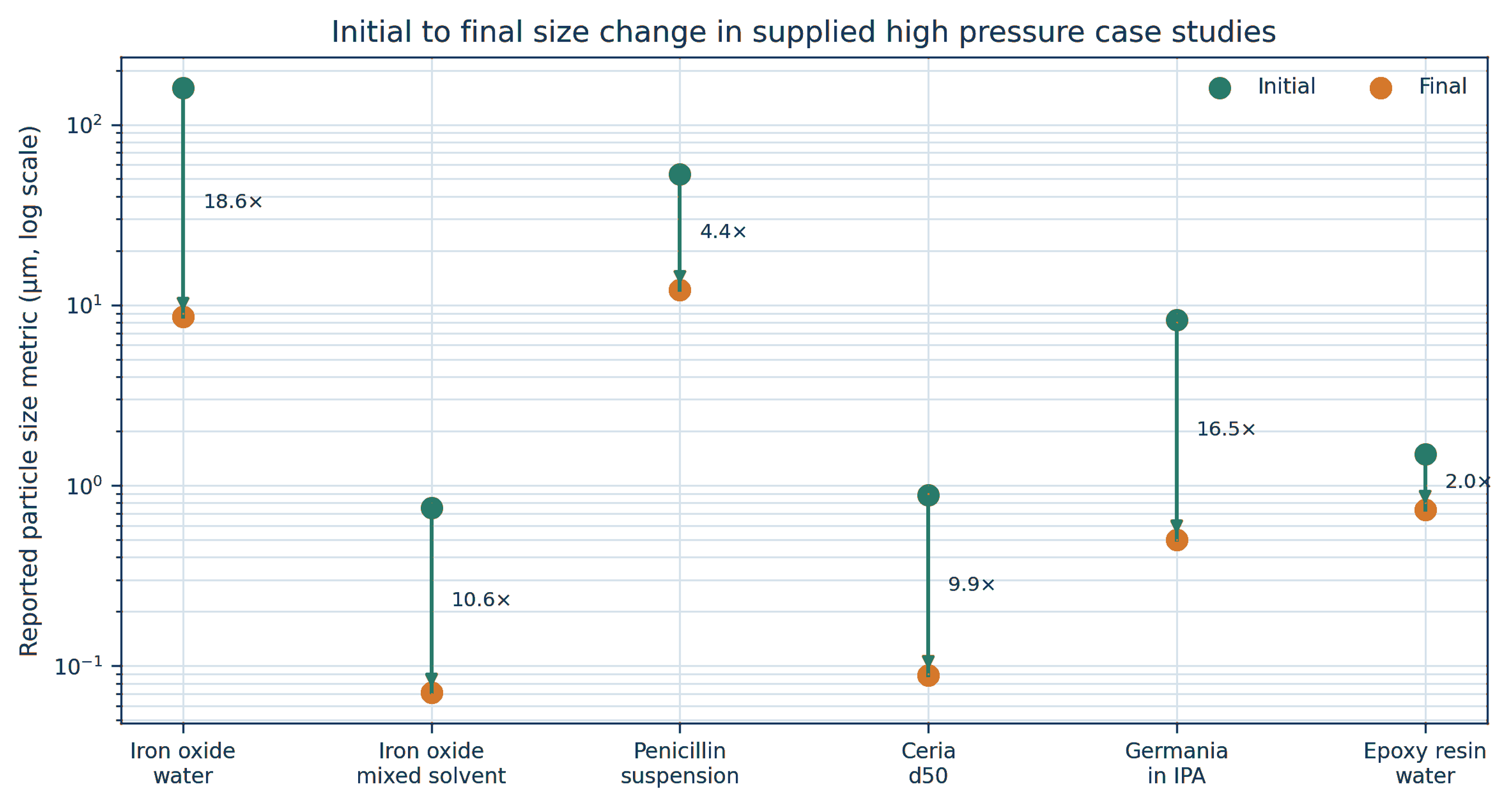
where Fd is the deagglomeration factor, dx,0 is the initial value of a specified particle size metric, and dx, f is its final value. For the water-based iron oxide test, Fd = 18.6. The factor is a reporting metric, not a mechanistic constant, and it is valid only when the same analytical method and weighting basis are used before and after processing.
Figure 8.13. Mean size and optical transmittance reported for 5 wt% iron oxide in water before and after 40 minutes at 5,000 psi [48]Source: Arisdyne Systems. High Pressure Cavitation of Iron Oxide in Water, 16 November 2009.
*[Figure 8.13](#figure-8-13). Mean size and optical transmittance reported for 5 wt% iron oxide in water before and after 40 minutes at 5,000 psi [48].*
Another data sheet describes iron oxide dispersed in a toluene and water mixture. Five passes through an M 110Y processor at 23,000 psi reduced the reported mean size from approximately 750 nm to 71 nm [49]. The sheet prints 15.86 MPa beside 23,000 psi; the correct pressure conversion is 158.6 MPa. This correction is important because pressure based energy and scale calculations would otherwise be low by a factor of ten.
Figure 8.14. Initial and final size metrics for selected supplied high-pressure case studies. Vertical arrows show the direction of size reduction, and labels show the deagglomeration factor defined by Equation (8.1) [48-54]Sources: Arisdyne Systems [48] and Microfluidics reports [49-54], as cited in the source document.
*[Figure 8.14](#figure-8-14). Initial and final size metrics for selected supplied high-pressure case studies. Vertical arrows show the direction of size reduction, and labels show the deagglomeration factor defined by Equation (8.1) [48-54].*
Table 8.5 summarizes the principal operating conditions and reported results. Pressure and pass count alone do not explain the different responses because feed strength, solids concentration, liquid viscosity, chamber geometry, and analytical basis vary substantially.
*Table 8.5. Selected high pressure particle processing results from supplied reports.*
| Material and medium | Solids | Pressure | Exposure | Initial metric | Final metric | Reduction | Source type |
|---|---|---|---|---|---|---|---|
| Iron oxide in water | 5 wt% | 34.47 MPa; 5,000 psi | 40 min; about 16 passes | Mean 160.23 µm | Mean 8.6 µm | 94.6% | Internal report [48] |
| Iron oxide in toluene and water | Not stated | 158.6 MPa; 23,000 psi | 5 passes | Mean 0.750 µm | Mean 0.071 µm | 90.5% | Manufacturer sheet [49] |
| Penicillin suspension | Not stated | 124.1 MPa; 18,000 psi | 1 pass | Mean 53 µm | Mean 12.1 µm | 77.2% | Manufacturer sheet [50] |
| Ceria in water, pH about 2.5 | 12 wt% | 158.6 MPa; 23,000 psi | 2 passes | d50 0.885 µm | d50 0.089 µm | 89.9% | Manufacturer test report [51] |
| Germania in isopropyl alcohol | 10 wt% | 158.6 MPa; 23,000 psi | 1 pass | Mean 8.301 µm | Mean 0.502 µm | 94.0% | Manufacturer sheet [52] |
| Bisphenol epoxy resin in water | 60 wt% | 68.95 MPa; 10,000 psi | 15 passes | Mean 1.486 µm | Mean 0.733 µm | 50.7% | Manufacturer sheet [54] |
### 8.12 Ceria and germania oxide systems
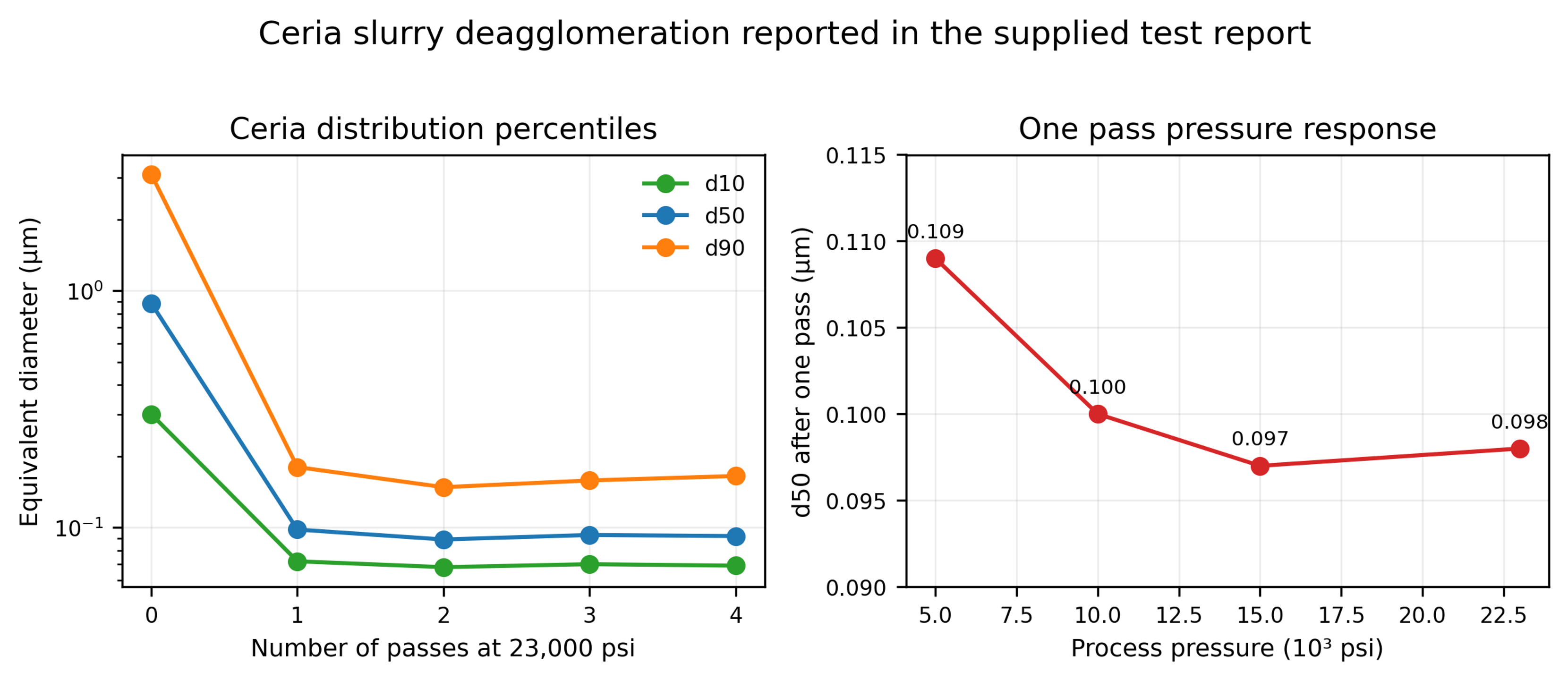
Additional ceria data provide a useful distinction between pressure response and pass response. A 12 wt% ceria slurry at pH about 2.5 had initial D₁₀, D₅₀, and D₉₀ values of 0.301, 0.885, and 3.100 µm, respectively. At 23,000 psi, the first pass reduced these values to 0.072, 0.098, and 0.180 µm. The minimum reported D₅₀ and D₉₀ values occurred after the second pass, at 0.089 and 0.148 µm, followed by small fluctuations during passes three and four [51]. The result indicates that most weak clusters failed during the first exposure, while the remaining coarse population approached an endpoint controlled by stronger contacts, reattachment, or measurement variation.
Figure 8.15. Ceria size percentiles versus pass count at 23,000 psi and one pass D₅₀ versus pressure [51]Source: Microfluidics Technology Center. Ceria Water Slurry Deagglomeration Test Report, undated supplied report.
*[Figure 8.15](#figure-8-15). Ceria size percentiles versus pass count at 23,000 psi and one pass D₅₀ versus pressure [51].*
The one pass median diameter changed only from D₅₀ = 0.109 µm at 5,000 psi to approximately 0.097 to 0.100 µm between 10,000 and 23,000 psi. Thus, once the chamber generated sufficient stress to disrupt the dominant agglomerates, further pressure increase produced limited additional change in the median. The upper tail and product damage should be monitored before selecting the highest pressure.
*Table 8.6. Ceria particle size results. [51].*
| **Pressure** | **Passes** | (µm) | (µm) | (µm) |
|--------------|------------|-------------------------|-------------------------|-------------------------|
| Control | 0 | 0.301 | 0.885 | 3.100 |
| 23,000 psi | 1 | 0.072 | 0.098 | 0.180 |
| 23,000 psi | 2 | 0.068 | 0.089 | 0.148 |
| 23,000 psi | 3 | 0.070 | 0.093 | 0.158 |
| 23,000 psi | 4 | 0.069 | 0.092 | 0.165 |
| 15,000 psi | 1 | 0.072 | 0.097 | 0.169 |
| 10,000 psi | 1 | 0.074 | 0.100 | 0.171 |
| 5,000 psi | 1 | 0.078 | 0.109 | 0.220 |
The germania data sheet reports a 10 wt% GeO₂ suspension in isopropyl alcohol. One pass at 23,000 psi reduced the mean size from 8.301 to 0.502 µm and D₉₀ from 14.469 to 0.612 µm [52]. The large reduction in both the mean and the coarse tail is consistent with extensive agglomerate disruption or fracture of brittle structures. Processing a flammable solvent at 158.6 MPa requires equipment specifically rated for the solvent, pressure, electrical classification, seal compatibility, and controlled heat removal. The reported result is not a general authorization to process isopropyl alcohol in an arbitrary cavitation unit.
### 8.13 Pharmaceutical crystals, concentrated resins, and equipment scale
A penicillin suspension processed once at 18,000 psi showed a reported mean size reduction from 53 to 12.1 µm [50]. This response after one pass is useful for preliminary equipment sizing, but pharmaceutical application requires additional verification of assay, polymorphic form, crystal habit, dissolution, sterility or bioburden controls, and excipient stability. A size target alone is not a complete pharmaceutical specification.
The 60 wt% bisphenol epoxy resin and water dispersion responded much more gradually. Fifteen passes at 10,000 psi reduced the reported mean size from 1.486 to 0.733 µm [54]. The modest factor of 2.03 is consistent with the combined effects of high dispersed phase concentration, increased viscosity, restricted bubble growth, and reattachment driven by collisions. In such systems, dilution studies and formulation optimization may be more effective than simply increasing pass count.
Equipment scale should be defined by pressure history, critical passage geometry, chamber material, flow per chamber, cooling capacity, and pass distribution rather than by machine designation alone. Parallel chambers can increase throughput, but every branch must receive the same pressure and must remain free of partial plugging. Abrasive oxide service also requires scheduled inspection of nozzles, seats, intensifier seals, and downstream metal contamination.
### 8.14 Carbon nanotube bundle separation and aspect ratio control
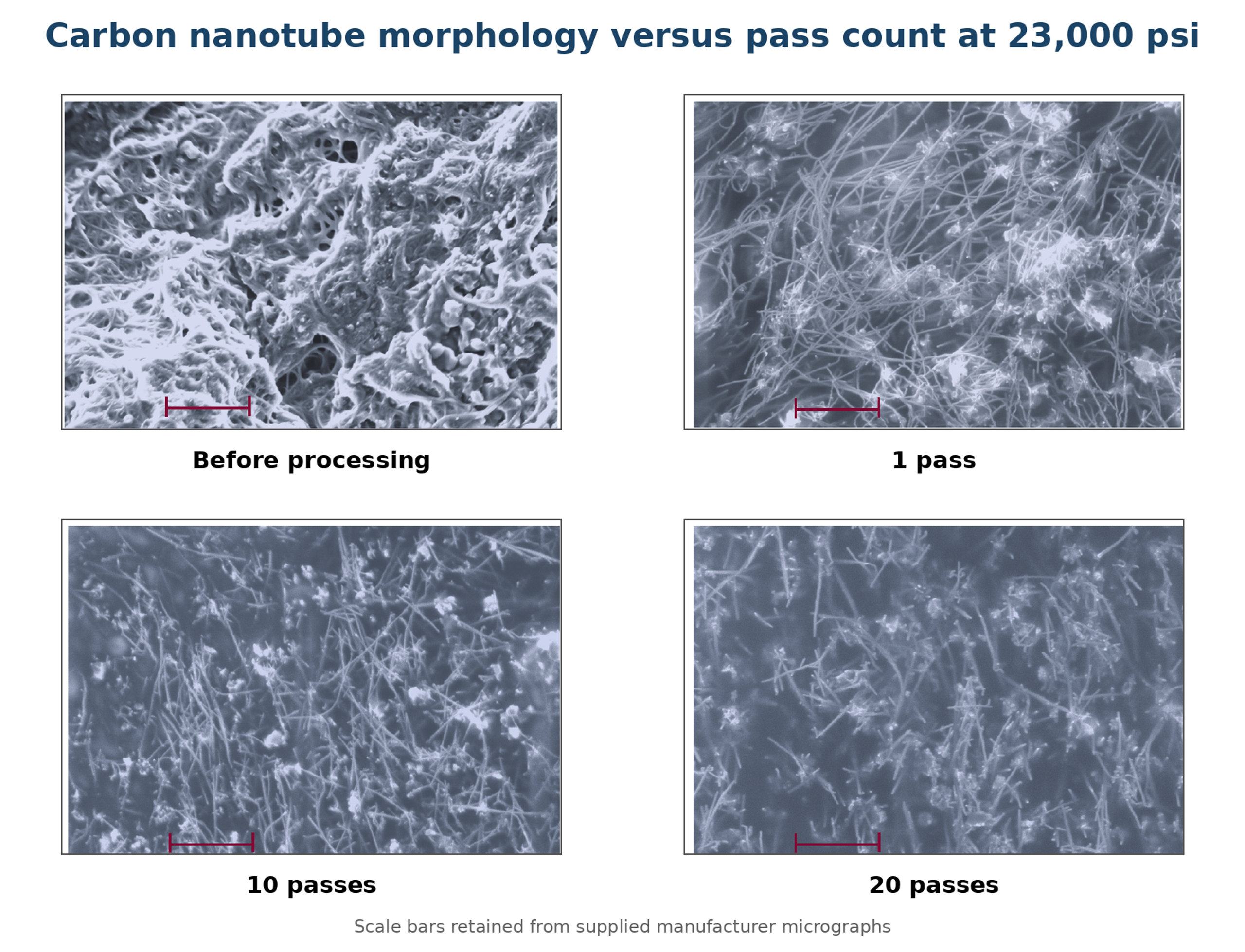
Carbon nanotubes illustrate the difference between successful deagglomeration and excessive structural damage. A manufacturer data sheet reports that one pass at 23,000 psi separated dense nanotube bundles, whereas 10 and 20 passes progressively shortened the visible nanotube population [53]. The reported chamber shear rate was 5.9 million s⁻¹. The first pass was therefore beneficial for bundle opening, but continued exposure shifted the mechanism toward tube scission and aspect ratio loss.
Figure 8.16. Carbon nanotube micrographs before processing and after 1, 10, and 20 passes. One pass opened the bundles, while additional passes shortened the visible nanotubes [53]Source: Microfluidics Corporation. Carbon Nanotubes: Deagglomeration and Length Reduction, 2005.
*[Figure 8.16](#figure-8-16). Carbon nanotube micrographs before processing and after 1, 10, and 20 passes. One pass opened the bundles, while additional passes shortened the visible nanotubes [53].*
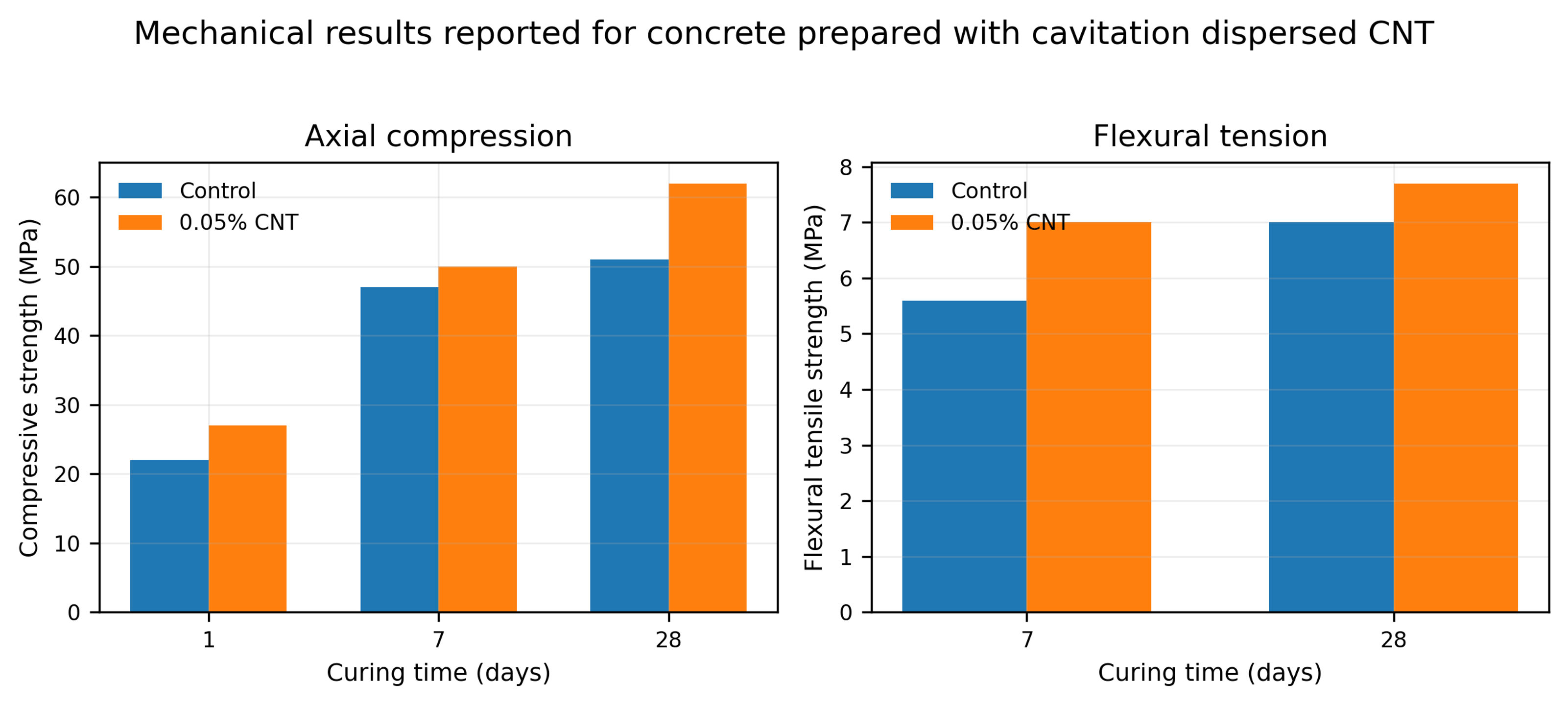
A separate article describes a 30 L hydrodynamic cavitation loop for dispersing multilayer carbon nanotubes in water containing a polycarboxylate superplasticizer. The reported flow was 1.15 L s⁻¹, motor power was 3 kW, treatment time was 60 minutes, and the suspension completed approximately 100 to 105 cycles through a passive cavitation disperser [56]. The resulting liquid was used to prepare concrete containing nanotubes at 0.05 percent of cement mass.
Figure 8.17. Mechanical results reported for concrete prepared with cavitation dispersed carbon nanotubes [56]Source: Gusev BV, Petrunin SY. Cavitation dispersion of carbon nanotubes and modification of cement systems. Nanotechnologies in Construction, 2014.
*[Figure 8.17](#figure-8-17). Mechanical results reported for concrete prepared with cavitation dispersed carbon nanotubes [56].*
*Table 8.7. Reported concrete strength with and without 0.05 percent carbon nanotubes. [56].*
| **Mixture** | **Compressive 1 day (MPa)** | **Compressive 7 days (MPa)** | **Compressive 28 days (MPa)** | **Flexural 28 days (MPa)** |
|-------------|-----------------------------|------------------------------|-------------------------------|----------------------------|
| Control | 22 | 47 | 51 | 7.0 |
| 0.05% CNT | 27 | 50 | 62 | 7.7 |
At 28 days, the reported compressive strength increased from 51 to 62 MPa and flexural strength increased from 7.0 to 7.7 MPa. These results are consistent with improved nanotube distribution, but the nanotube addition itself, superplasticizer interactions, curing, air content, and batch variability also affect strength. A rigorous validation should include dispersion microscopy, rheology, replicate specimens, and a control prepared with the same dispersant and processing history but without nanotubes.
### 8.15 Plant raw materials, controlled comminution, and mass transfer area
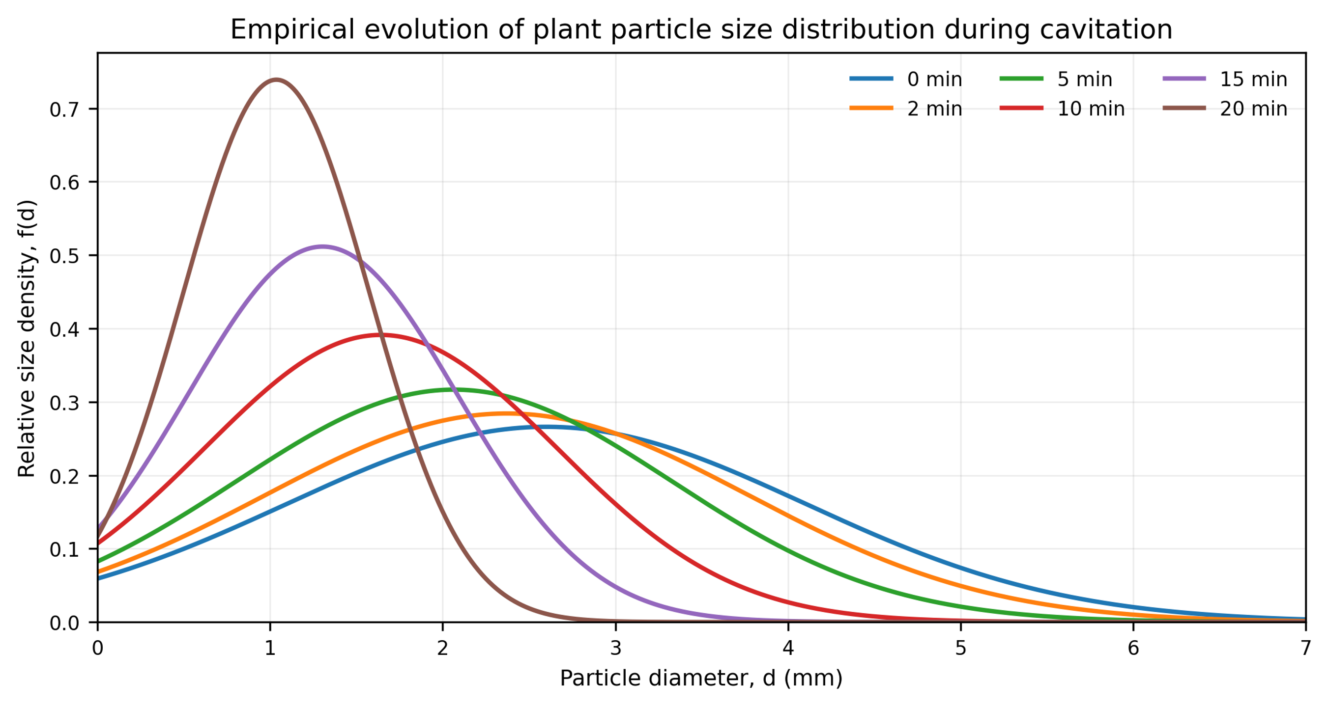
Vitenko and Zaretska studied white and black mulberry leaves in a static cavitation device consisting of a circulation loop and a Venturi type working section with an adjustable truncated cone. Ground leaves and extractant were charged at a mass ratio of 1 to 10 and processed for 2, 5, 10, 15, or 20 minutes [55]. The objective was to increase the solid-liquid mass transfer area enough to accelerate extraction without producing excessive fines that increase turbidity and complicate separation.
The authors represented the measured particle diameter distribution by a normal density function:
(8.2)
where *f*(*d*) is the relative density of particle diameters, *d* is particle diameter in millimeters, is the fitted mean diameter, and is the fitted standard deviation. For the reported material and operating range, the time dependence was approximated by:
(8.3)
(8.4)
where τ is the cavitation processing time in minutes. These empirical relations apply only to the specified mulberry feed, pretreatment, liquid ratio, and device. They should not be extrapolated beyond the 0 to 20 minute test interval without new measurements.
Figure 8.18. Empirical evolution of the plant particle diameter distribution calculated from Equations (8.2) to (8.4) [55]Source: Vitenko TM, Zaretska TV. Evaluation of cavitation comminution of plant raw materials using white and black mulberry, 2011.
*[Figure 8.18](#figure-8-18). Empirical evolution of the plant particle diameter distribution calculated from Equations (8.2) to (8.4) [55].*
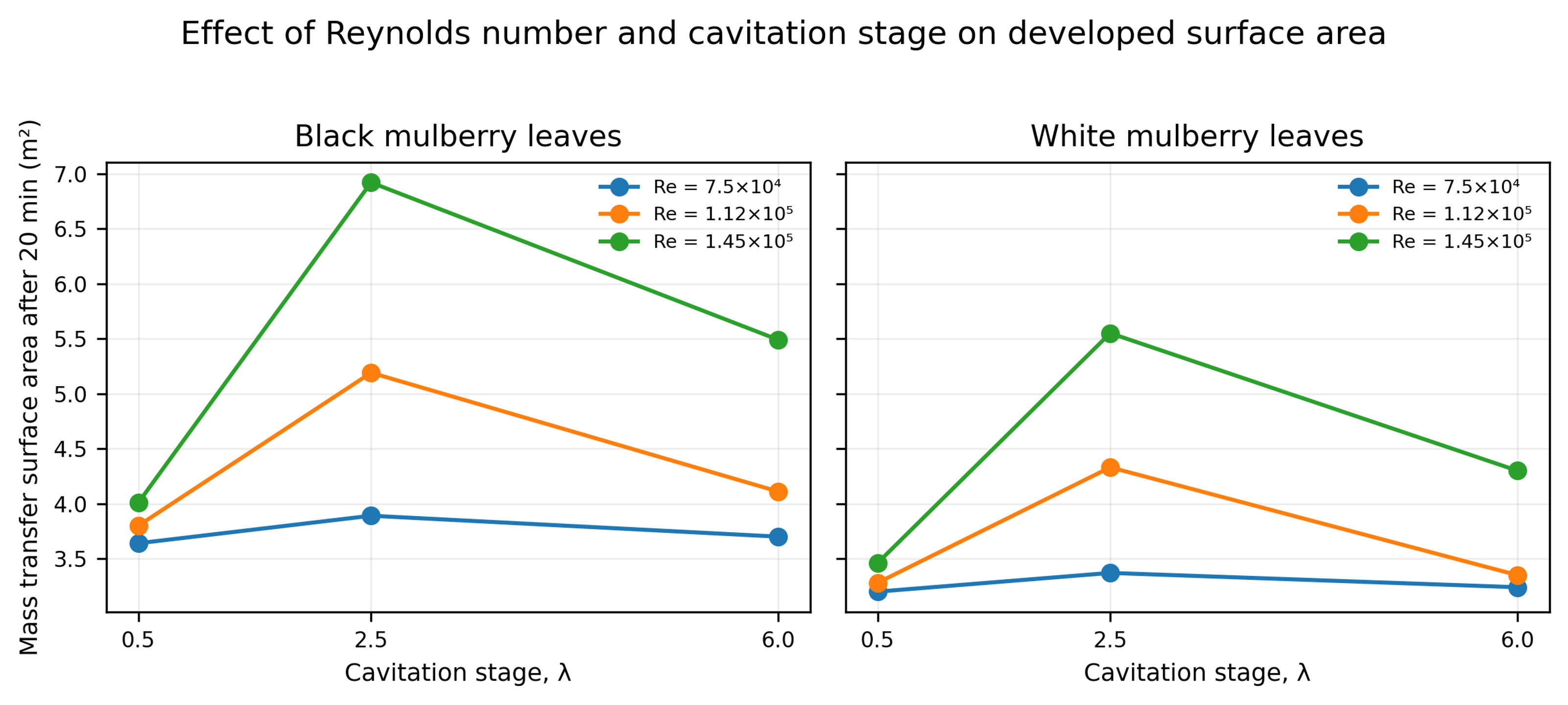
The strongest surface development occurred at *Re* = 1.45 × 10⁵ and λ = 2.5. After 20 minutes, the reported mass transfer area increased from 3.62 to 6.92 m² for black mulberry and from 3.16 to 5.55 m² for white mulberry. These changes correspond to area increases of approximately 91 and 76 percent. At λ = 0.5, comminution was limited, whereas λ = 6 produced less surface area than the intermediate stage. The nonmonotonic response is consistent with a change from productive collapse to an overdeveloped cavity field, shielding, or altered residence in the most effective collapse zone.
Figure 8.19. Final mass transfer surface area after 20 minutes as a function of Reynolds number and cavitation stage for black and white mulberry leaves [55]Source: Vitenko TM, Zaretska TV. Evaluation of cavitation comminution of plant raw materials using white and black mulberry, 2011.
*[Figure 8.19](#figure-8-19). Final mass transfer surface area after 20 minutes as a function of Reynolds number and cavitation stage for black and white mulberry leaves [55].*
*Table 8.8. Change in plant mass transfer surface area after 20 minutes. Source: [55].*
| **Reynolds number** | **Cavitation stage λ** | **Black mulberry, m²** | **Black area ratio** | **White mulberry, m²** | **White area ratio** |
|---------------------|------------------------|------------------------|----------------------|------------------------|----------------------|
| 7.5 × 10⁴ | 0.5 | 3.62 to 3.64 | 1.01 | 3.16 to 3.20 | 1.01 |
| 7.5 × 10⁴ | 2.5 | 3.62 to 3.89 | 1.07 | 3.16 to 3.37 | 1.07 |
| 7.5 × 10⁴ | 6 | 3.62 to 3.70 | 1.02 | 3.16 to 3.24 | 1.03 |
| 1.12 × 10⁵ | 0.5 | 3.62 to 3.80 | 1.05 | 3.16 to 3.28 | 1.04 |
| 1.12 × 10⁵ | 2.5 | 3.62 to 5.19 | 1.43 | 3.16 to 4.33 | 1.37 |
| 1.12 × 10⁵ | 6 | 3.62 to 4.11 | 1.14 | 3.16 to 3.35 | 1.06 |
| 1.45 × 10⁵ | 0.5 | 3.62 to 4.01 | 1.11 | 3.16 to 3.46 | 1.09 |
| 1.45 × 10⁵ | 2.5 | 3.62 to 6.92 | 1.91 | 3.16 to 5.55 | 1.76 |
| 1.45 × 10⁵ | 6 | 3.62 to 5.49 | 1.52 | 3.16 to 4.30 | 1.36 |
The article also reports that formation of particles below 1 mm increased liquid turbidity and complicated clarification. This is a practical reminder that the optimum extraction condition may be below the condition that maximizes newly created area. Product recovery, filtration, centrifugation, and sensory or optical quality must be included in the optimization criterion.
### 8.16 Cross case interpretation and endpoint selection
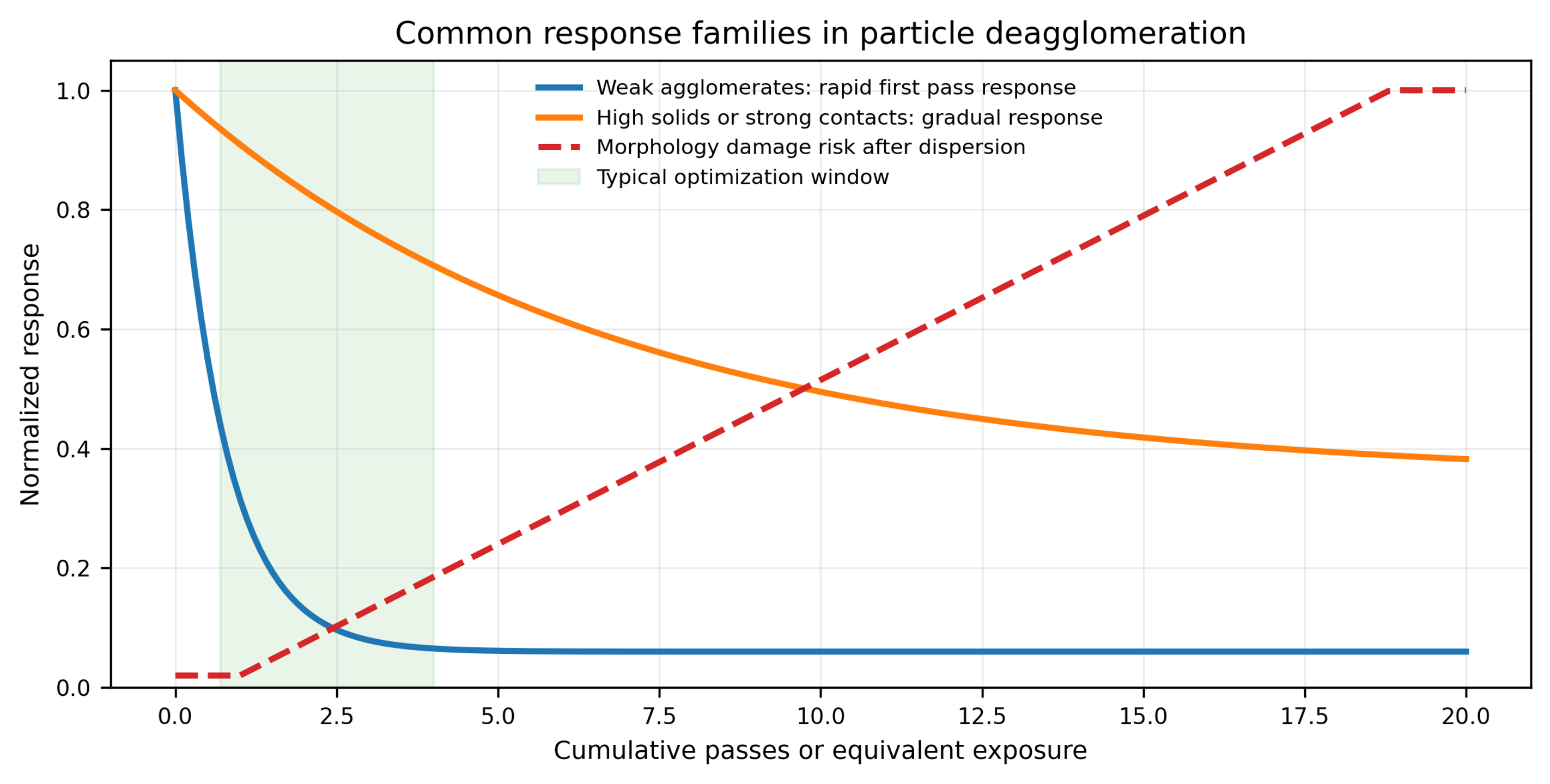
Many data sets that vary with pass count can be described empirically by an asymptotic endpoint model:
(8.5)
where dₓ(N) is the selected size metric after N passes, dₓ,∞ is the asymptotic value for the specified formulation and device, and kₓ is an empirical pass response constant. The equation is not a universal breakage law. It is a compact way to quantify the large first pass change, declining incremental benefit, and practical endpoint observed for ZnO, ceria, soy solids, and other feeds.
Figure 8.20. Common response families in particle deagglomeration. Weak agglomerates may show a rapid first pass response, concentrated or strongly bonded systems may respond gradually, and morphology damage risk can increase after the dispersion objective has already been reached [58]Source: Kozyuk O. Hydrodynamic Cavitation. Unpublished technical manuscript and supporting data, 2026.
*[Figure 8.20](#figure-8-20). Common response families in particle deagglomeration. Weak agglomerates may show a rapid first pass response, concentrated or strongly bonded systems may respond gradually, and morphology damage risk can increase after the dispersion objective has already been reached [58].*
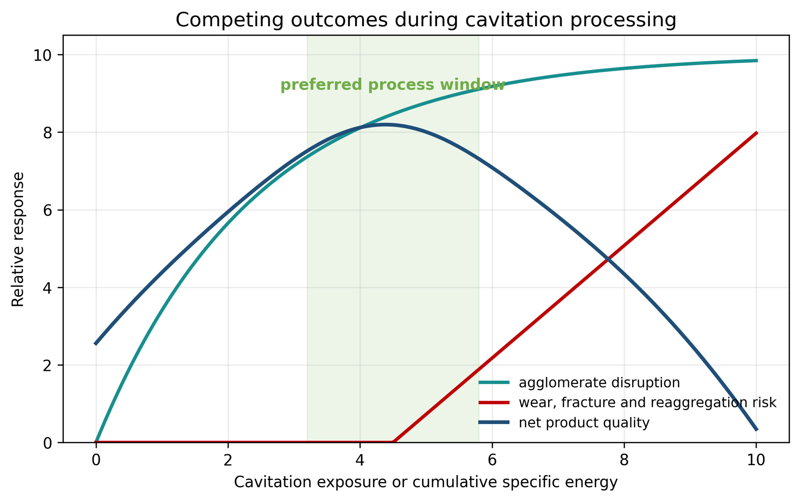
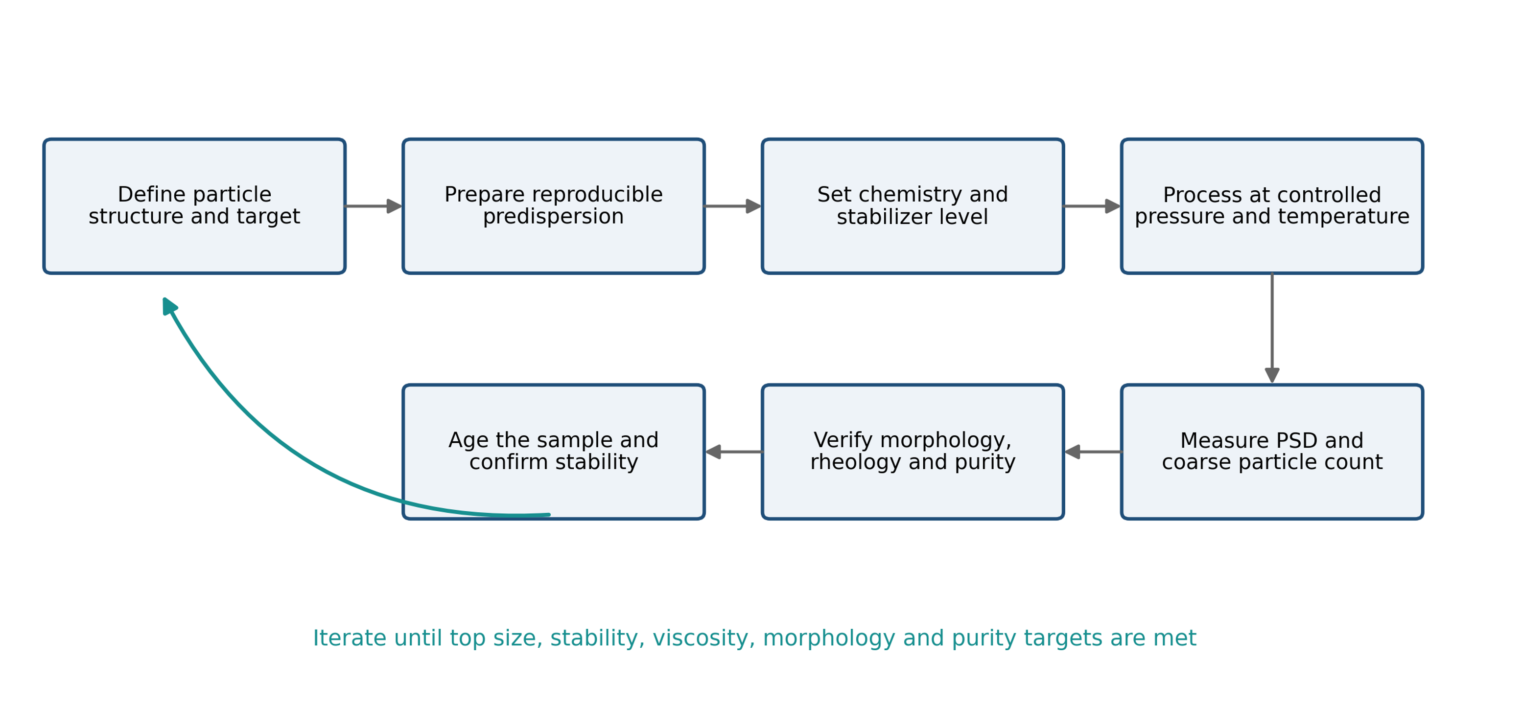
Across the supplied cases, four recurring conclusions emerge. First, the first effective pass often removes most weak agglomerates. Second, high solids loading and viscosity can shift the process toward gradual erosion and repeated exposure. Third, the median may reach a plateau while the coarse tail or morphology continues to change. Fourth, carbon nanotube, fiber, and flake systems require an explicit aspect ratio or length specification because additional processing can improve dispersion while simultaneously degrading function. The process endpoint should therefore be determined from particle size, coarse particle count, aged stability, rheology, morphology, contamination, and application performance rather than from pressure or pass count alone.
## 9 Process variables and optimization
### 9.1 Pressure drop and cavitation number
Increasing pressure drop generally increases jet velocity, lowers cavitation number, and increases the probability of severe collapse. The response usually exhibits diminishing returns. Weak clusters are removed first, while the remaining structures are stronger or the product reaches an endpoint limited by stability. Excess pressure can increase wear and temperature without improving aged particle size.
The correct objective is the minimum pressure and cumulative exposure that satisfy the particle size, stability, morphology, purity, and throughput requirements. A process should not be optimized by the smallest immediate value alone.
### 9.2 Geometry and collapse location
Passage diameter, the ratio of length to diameter, contraction profile, recovery angle, downstream chamber, and wall proximity determine where cavities form and collapse. For dispersion, the preferred collapse region is one where particles are present, and wall erosion is manageable. A short microchannel can move collapse downstream, while a long channel may sustain a vapor cavity or erode internally [23–25].
A small passage increases local velocity and stress but also increases plugging and contamination risk. For feeds with a broad coarse tail, a staged system is often more robust than a single fine restriction.
### 9.3 Number of passes and residence time distribution
The first pass often produces the largest improvement, as shown by ZnO and soy slurry. Later passes target stronger structures and deliver smaller incremental reductions. The optimum pass count is the minimum that meets both immediate and aged specifications.
In a recirculating tank, the actual exposure distribution must be considered. A well-mixed tank provides statistical redistribution, while poor mixing leaves untreated material and repeatedly processes fluid near the return. A once-through or series arrangement provides tighter exposure but may require more devices or higher pressure.
### 9.4 Solids loading and viscosity
Higher solids loading increases throughput per unit liquid and collision frequency. It also raises viscosity, pressure loss, plugging tendency, and the probability of reaggregation. Viscous damping can suppress bubble growth and change cavity structure. A formulation that disperses successfully at 0.1 wt% may not behave similarly at 40 wt%.
Possible strategies include predilution, staged solids addition, controlled heating, a larger first stage, or processing in a carrier followed by letdown. Final validation must be performed at the intended production solids and temperature.
### 9.5 Surface chemistry and dispersant level
Fresh surface must be stabilized rapidly. Important variables include pH, ionic strength, counterion identity, solvent polarity, surfactant concentration, polymer molecular mass, adsorption kinetics, and competitive adsorption. A useful experimental matrix combines cavitation intensity with dispersant concentration. Higher pressure may improve immediate size but worsen aged size when dispersant is insufficient.
### 9.6 Temperature, dissolved gas, and nuclei
Higher temperature raises vapor pressure and usually lowers viscosity. Cavitation may begin more readily, but increased vapor content can cushion collapse. Temperature also affects adsorption, solubility, polymer conformation, and chemical stability. Inlet and outlet temperatures should be recorded at the reactor, not only in the tank.
Dissolved and entrained gas influence both bubble number and collapse severity. Noncondensable gas cushions collapse but can increase the number of cavities. Degassing may produce fewer but more severe vapor collapses. Gas addition can create a dense, milder bubble population and increase foam. The optimum depends on whether shock intensity, mixing, or gas-liquid interfacial area controls the process.
### 9.7 Erosion, contamination, and morphology preservation
Cavitation erosion can release metal, ceramic, or polymer debris from nozzles, valves, and downstream surfaces. Risk is highest where bubbles repeatedly collapse near a wall. Replaceable inserts, hard materials, smoother recovery, and relocation of the collapse zone can reduce contamination. Wear should be assessed by mass loss, dimensional inspection, and elemental analysis of product and blanks.
Morphology preservation must be verified for flakes, fibers, hollow particles, coated particles, and soft crystals. A process that produces a low value may be unacceptable if it shortens carbon fibers, destroys silver flake aspect ratio, removes a functional coating, or changes a pharmaceutical polymorph.
Figure 9.1. Conceptual balance among agglomerate disruption, product quality, and damage risk [58]Source: Kozyuk O. Hydrodynamic Cavitation. Unpublished technical manuscript and supporting data, 2026.
*[Figure 9.1](#figure-9-1). Conceptual balance among agglomerate disruption, product quality, and damage risk [58].*
*Table 9.1. Directional effects of major process variables.*
| **Variable increased** | **Likely beneficial effect** | **Potential adverse effect** |
|--------------------------|---------------------------------------------------|----------------------------------------------------------|
| Pressure drop | Higher velocity and stronger cavitation | Wear, heating, fracture, reaggregation |
| Number of passes | Greater probability of disrupting strong clusters | Diminishing returns, contamination, thermal exposure |
| Solids loading | Higher production rate and more collisions | Viscosity, plugging, poor exposure uniformity |
| Temperature | Lower viscosity and easier inception | Degradation, desorption, vapor cushioning |
| Dissolved gas | More nuclei and bubbles | Collapse cushioning, foam, oxidation |
| Dispersant concentration | Faster stabilization of fresh surface | Bridging, viscosity increase, altered product properties |
| Smaller passage | Higher local velocity and stress | Plugging and accelerated erosion |
| Faster pressure recovery | More severe collapse | Wall damage and morphology loss |
### 9.8 Experimental design
A useful development design includes pressure, geometry, pass count, solids concentration, temperature, dispersant level, and gas condition. Responses should include , , span, coarse particle count, viscosity, aged size, morphology, and at least one purity or functional measure. Factor interactions should be expected. Statistical replication is particularly important when nuclei condition and sampling vary.
## 10 Scale-up, equipment selection, and troubleshooting
### 10.1 Parameters to preserve
No single similarity parameter guarantees scale up. A robust strategy preserves the variables that control the specific formulation:
- Cavitation number or a validated geometry specific inception margin.
- Local pressure drop profile and pressure recovery rate.
- Critical passage dimension relative to the incoming coarse tail.
- Local dissipation rate and collapse exposure.
- Nominal passes and residence time distribution.
- Solids loading, viscosity, surface tension, vapor pressure, and gas content.
- Inlet and outlet temperature.
- Stabilizer amount relative to newly created surface area.
- Wear material and collapse location.
Figure 10.1. Representative operating domains for selected cavitation dispersion devices. Boundaries are conceptual, not universal design limits [58]Source: Kozyuk O. Hydrodynamic Cavitation. Unpublished technical manuscript and supporting data, 2026.
*[Figure 10.1](#figure-10-1). Representative operating domains for selected cavitation dispersion devices. Boundaries are conceptual, not universal design limits [58].*
### 10.2 Throughput scaling by numbering up
For parallel geometrically identical passages, throughput can be increased by adding passages while preserving the pressure history in each element. This numbering up approach is often more reliable than enlarging one micro orifice because enlargement changes velocity gradients, cavity structure, and nuclei behavior. The manifold must distribute flow uniformly and avoid dead legs.
Figure 10.2. Numbering up of identical critical passages in a recirculating production loop [58]Source: Kozyuk O. Hydrodynamic Cavitation. Unpublished technical manuscript and supporting data, 2026.
*[Figure 10.2](#figure-10-2). Numbering up of identical critical passages in a recirculating production loop [58].*
For larger static reactors, scale up can increase the number of holes or stages while preserving hole diameter and pressure drop. For dynamic processors, tip speed, gap, stage count, and power per unit throughput are relevant, but equal tip speed does not guarantee equal cavity cloud structure. Pilot testing remains necessary.
### 10.3 Heat removal
Even when particle breakup is highly localized, most supplied power ultimately becomes heat. At steady state, the required heat exchanger duty is approximately:
(10.1)
where is motor power transferred to the process and the second term represents any allowable sensible temperature rise. The exchanger should be sized from measured power and temperature, not an assumed cavitation efficiency.
### 10.4 Stagewise development procedure
Figure 10.3. Recommended development workflow for cavitation-assisted particle dispersing [58]Source: Kozyuk O. Hydrodynamic Cavitation. Unpublished technical manuscript and supporting data, 2026.
*[Figure 10.3](#figure-10-3). Recommended development workflow for cavitation-assisted particle dispersing.*
A practical scale-up sequence is:
- Establish a reproducible feed preparation and analytical method.
- Define the primary particle, aggregate, agglomerate, and floc structure.
- Determine the minimum pressure and pass count that meet immediate size targets.
- Optimize stabilizer level and verify aged size and rheology.
- Confirm morphology, crystal structure, and purity.
- Measure temperature rise, pressure pulsation, flow, and wear.
- Increase batch volume while preserving the same critical reactor.
- Add parallel passages or stages before changing critical geometry.
- Verify manifold balance and actual pass distribution.
- Repeat aging, functional, cleaning, and contamination tests at production scale.
*Table 10.1. Scale-up verification checks.*
| **Check** | **Laboratory evidence** | **Production verification** |
|----------------------|---------------------------------------------|-----------------------------------------------------|
| Cavitation inception | Pressure, flow, acoustic or visual response | Same operating margin at every parallel element |
| Exposure | Pass count and loop residence time | Tracer test or validated recirculation model |
| Product size | PSD and microscopy | At line PSD using retained reference method |
| Stabilization | Aged PSD, zeta potential, rheology | Storage, thermal cycling, and shipping simulation |
| Heat | Reactor inlet and outlet temperature | Heat exchanger duty and steady state balance |
| Wear | Short duration inspection and blanks | Campaign length elemental and dimensional checks |
| Cleanability | Bench cleaning test | Full skid drainability and validated cleaning cycle |
### 10.5 Troubleshooting
*Table 10.2. Troubleshooting guide.*
| **Observation** | **Probable cause** | **Corrective action** |
|----------------------------------------------------------|--------------------------------------------------------------------------------------------|------------------------------------------------------------------------------------------------|
| Little size reduction | Cavitation not established, recovery too slow, agglomerates too strong, viscosity too high | Verify pressure and flow, modify geometry, increase passes, predilute, use staged processing |
| decreases but remains high | Bypass, poor tank mixing, plugging, small resistant population | Improve recirculation, inspect passages, add a coarse first stage, extend exposure cautiously |
| Size improves immediately but rebounds | Inadequate stabilizer, unfavorable pH or ionic strength, high collision rate | Add stabilizer before processing, adjust chemistry, reduce handling intensity after processing |
| Viscosity rises sharply | Increased surface area, network formation, excessive dispersion, temperature change | Optimize dispersant, reduce exposure, control temperature, verify solids concentration |
| Viscosity decreases but conductivity or strength worsens | Flake or fiber aspect ratio damage | Reduce pressure or passes, use larger passages, verify morphology |
| Metal concentration increases | Cavitation erosion or pump wear | Relocate collapse zone, change materials, install replaceable inserts, reduce severity |
| Coarse particles increase | Cavitation induced agglomeration or contamination | Review chemistry, gas content, pump suction, and stabilization; reduce cavitation |
| Poor repeatability | Variable nuclei, gas entrainment, temperature, sampling, or analytical dilution | Standardize degassing, tank level, temperature, sampling, and measurement protocol |
| Passage plugs | Incoming tail too large, sedimentation, poor premixing | Add screening or a coarse stage, increase passage size, improve tank suspension |
| Excessive foaming | Gas entrainment, surfactant, return line above liquid level | Submerge return, improve degassing, adjust formulation, reduce suction leakage |
## 11 Conclusions
Hydrodynamic cavitation provides a versatile, media-free approach to the dispersion of agglomerated particles and, at greater severity, to controlled comminution or exfoliation. Its performance results from the combined action of extensional flow, viscous stress, inertial turbulence, bubble-induced particle motion, shock waves, liquid microjets, and interparticle collisions. Because these mechanisms act at different locations and length scales, neither pressure drop nor average power density alone is an adequate descriptor of process severity.
The reviewed case studies demonstrate substantial reductions in suspended-object size for ZnO, bentonite, silver, alumina, titania, iron oxide, ceria, germania, penicillin crystals, soy solids, and plant raw materials. They also demonstrate production of fine silicon fractions, exfoliation of graphite, improved carbon-nanotube distribution, and the possibility of undesirable agglomeration or morphology damage. Manufacturer and internal reports are useful for defining preliminary operating ranges, but their conclusions require confirmation by controlled analytical methods and application-specific performance tests.
The most reliable scale-up strategy preserves the critical pressure history and passage geometry, controls the pass and residence-time distributions, provides adequate heat removal, and treats erosion and contamination as design variables. Throughput should be increased by parallelization or staged processing whenever practical. The engineering endpoint is not the smallest immediate particle size, but the narrowest stable distribution that satisfies functional performance while preserving morphology, purity, crystal structure, and economically acceptable throughput.
## Nomenclature
| **Symbol** | **Definition** | **SI unit or status** |
|----------------------------------------------------------|--------------------------------------------------------------------------------------|---------------------------------------|
| | Particle radius | m |
| | External particle area per unit mass | m² kg⁻¹ |
| | Hamaker constant | J |
| | Daughter size distribution from parent size | Model dependent |
| | Breakage number | Dimensionless |
| , | Sound speed in liquid and solid | m s⁻¹ |
| | Discharge coefficient | Dimensionless |
| | Structural coefficient in agglomerate strength relation | Dimensionless |
| | Specific heat capacity | J kg⁻¹ K⁻¹ |
| | Agglomerate characteristic size | m |
| | Load bearing building block size | m |
| | Hydrodynamic particle diameter | m |
| | Particle diameter | m |
| | Diameter below which 10 percent of the stated distribution occurs | m |
| | Volume weighted mean diameter | m |
| | Median diameter | m |
| | Diameter below which 90 percent of the stated distribution occurs | m |
| | Brownian diffusion coefficient | m² s⁻¹ |
| | Specific hydraulic energy for one pass | J kg⁻¹ |
| | Cumulative specific energy input | J kg⁻¹ |
| | Elementary charge | C |
| | van der Waals attractive force | N |
| | Characteristic interparticle bond force | N |
| | Capillary force | N |
| | Gravitational acceleration | m s⁻² |
| | Surface separation distance | m |
| | Ionic strength | mol m⁻³ or stated concentration basis |
| | Polytropic exponent or pass index, as defined | Dimensionless |
| | Boltzmann constant | J K⁻¹ |
| | Characteristic length or settling height | m |
| | Mass of solid | kg |
| | Estimated dispersant mass | kg |
| | Number density distribution | Model dependent |
| | Avogadro constant | mol⁻¹ |
| | Nominal number of passes | Dimensionless |
| | Pressure inside bubble | Pa |
| | Noncondensable gas pressure | Pa |
| | Liquid solid impact pressure | Pa |
| | Reference pressure for cavitation number | Pa |
| | Saturation vapor pressure | Pa |
| | Far field or recovered pressure | Pa |
| | Hydraulic power | W |
| | Motor power transferred to process | W |
| | Sedimentation Peclet number | Dimensionless |
| | Volumetric flow rate | m³ s⁻¹ |
| | Heat exchanger duty | W |
| | Instantaneous bubble radius | m |
| | Initial or maximum bubble radius | m |
| | Percent reduction in selected diameter | % |
| | Breakage frequency | s⁻¹ |
| | Particle size distribution span | Dimensionless |
| | Stokes number | Dimensionless |
| | Time | s |
| | Rayleigh collapse time | s |
| | Absolute temperature | K |
| | Liquid microjet velocity | m s⁻¹ |
| | Characteristic mean flow velocity | m s⁻¹ |
| | Batch volume | m³ |
| , , , | Interaction potentials | J |
| | Settling velocity | m s⁻¹ |
| AFM | Atomic force microscopy | Abbreviation |
| CFC | Controlled flow cavitation | Abbreviation |
| CFD | Computational fluid dynamics | Abbreviation |
| CMP | Chemical mechanical planarization | Abbreviation |
| DLS | Dynamic light scattering | Abbreviation |
| ICP | Inductively coupled plasma analysis | Abbreviation |
| PSD | Particle size distribution | Abbreviation |
| SEM | Scanning electron microscopy | Abbreviation |
| TEM | Transmission electron microscopy | Abbreviation |
| | Deagglomeration factor, initial selected diameter divided by final selected diameter | Dimensionless |
| *f*(*d*) | Relative probability density of plant particle diameter in Equation (8.2) | mm⁻¹ |
| | Fitted mean plant particle diameter in Equations (8.2) and (8.3) | mm |
| ; ; | Initial, final, and asymptotic value of selected particle size metric | m or stated unit |
| | Empirical pass response constant in Equation (8.5) | Pass⁻¹ |
| *Re* | Reynolds number | Dimensionless |
| IPA | Isopropyl alcohol | Abbreviation |
### Greek Letters
| **Symbol** | **Letter name** | **Meaning** | **SI unit or status** |
|------------------------------------|-----------------|--------------------------------------------------------------------------|-----------------------|
| | Alpha | Empirical coefficient relating jet momentum to effective collapse stress | Dimensionless |
| | Gamma | Adsorbed dispersant mass per unit area | kg m⁻² |
| | Gamma | Liquid surface tension | N m⁻¹ |
| | Delta p | Pressure drop across cavitation device | Pa |
| | Delta T | Adiabatic temperature rise | K |
| | Gamma dot | Kolmogorov strain rate | s⁻¹ |
| | Epsilon zero | Vacuum permittivity | F m⁻¹ |
| | Epsilon r | Relative permittivity | Dimensionless |
| | Epsilon a | Agglomerate porosity | Dimensionless |
| | Epsilon t | Turbulent energy dissipation rate per unit mass | m² s⁻³ |
| | Eta h | Overall hydraulic efficiency | Dimensionless |
| | Eta K | Kolmogorov microscale | m |
| | Theta | Contact angle | rad or degree |
| | Kappa | Inverse Debye screening length | m⁻¹ |
| | Kappa inverse | Debye screening length | m |
| | Mu | Dynamic viscosity | Pa s |
| | Nu | Kinematic viscosity | m² s⁻¹ |
| , , | Rho | Liquid, particle, and solid density | kg m⁻³ |
| | Sigma | Cavitation number | Dimensionless |
| | Sigma | Agglomerate tensile strength | Pa |
| | Tau | Effective collapse induced stress | Pa |
| | Tau | Characteristic flow time | s |
| | Tau | Kolmogorov time scale | s |
| | Tau | Particle relaxation time | s |
| | Tau | Applied external stress | Pa |
| | Tau | Inertial turbulent stress | Pa |
| | Tau | Viscous turbulent stress | Pa |
| | Psi | Surface potential | V |
| λ | Lambda | Cavitation stage used in the plant raw material study | Dimensionless |
| | Sigma d | Standard deviation of plant particle diameter distribution | mm |
| τ | Tau | Cavitation processing time in the plant raw material model | min |
## Bibliography
[1] Michel FC Jr, Kozyuk O. Hydrodynamic cavitation processing. In: Letcher TM, Scott JL, Patterson DA, editors. Chemical Processes for a Sustainable Future. Cambridge: Royal Society of Chemistry; 2015. pp. 84-142. doi: 10.1039/BK9781849739757-00084.
[2] Kozyuk OV. Particle size reduction and deagglomeration. Technical manuscript and supporting data supplied for this chapter; undated.
[3] Brennen CE. Cavitation and Bubble Dynamics. New York: Oxford University Press; 1995.
[4] Young FR. Cavitation. London: Imperial College Press; 1999.
[5] Plesset MS, Prosperetti A. Bubble dynamics and cavitation. Annual Review of Fluid Mechanics. 1977;9:145-185.
[6] Lauterborn W, Kurz T. Physics of bubble oscillations. Reports on Progress in Physics. 2010;73:106501. doi: 10.1088/0034-4885/73/10/106501.
[7] Blake JR, Gibson DC. Cavitation bubbles near boundaries. Annual Review of Fluid Mechanics. 1987;19:99-123.
[8] Yu J, Luo J, Li Y, Zhang Y. A review of bubble collapse near particles. International Journal of Fluid Engineering. 2024;1(2):020601. doi: 10.1063/5.0193451.
[9] Wolfrum B, Kurz T, Mettin R, Lauterborn W. Shock wave induced interaction of microbubbles and boundaries. Physics of Fluids. 2003;15(10):2916-2922. doi: 10.1063/1.1608938.
[10] Borkent BM, Arora M, Ohl CD, de Jong N, Versluis M, Lohse D, et al. The acceleration of solid particles subjected to cavitation nucleation. Journal of Fluid Mechanics. 2008;610:157-182.
[11] Zheng Y, Chen L, Liang X, Duan H. Numerical study of the interaction between a collapsing bubble and a movable particle in a free field. Water. 2020;12(12):3331. doi: 10.3390/w12123331.
[12] Zeiger BW, Suslick KS. Sonofragmentation of molecular crystals. Journal of the American Chemical Society. 2011;133(37):14530-14533. doi: 10.1021/ja205867f.
[13] Suslick KS. Sonochemistry. Science. 1990;247:1439-1445.
[14] Bałdyga J, Malik K. Selection and comparison of equipment for deagglomeration processes. Polish Journal of Chemical Technology. 2009;11(2):6-12. doi: 10.2478/v10026-009-0017-y.
[15] Biggs S. Aggregate structures and solid liquid separation processes. KONA Powder and Particle Journal. 2006;24:41-53. doi: 10.14356/kona.2006008.
[16] Ogi T, Zulhijah R, Iwaki T, Okuyama K. Recent progress in nanoparticle dispersion using bead mill. KONA Powder and Particle Journal. 2017;34:3-23. doi: 10.14356/kona.2017004.
[17] Li M, Azad M, Davé R, Bilgili E. Nanomilling of drugs for bioavailability enhancement: a holistic formulation process perspective. Pharmaceutics. 2016;8(2):17. doi: 10.3390/pharmaceutics8020017.
[18] Ishida N, Craig VSJ. Direct measurement of interaction forces between surfaces in liquids using atomic force microscopy. KONA Powder and Particle Journal. 2019;36:187-200. doi: 10.14356/kona.2019013.
[19] Hunter RJ. Foundations of Colloid Science. 2nd ed. Oxford: Oxford University Press; 2001.
[20] Mewis J, Wagner NJ. Colloidal Suspension Rheology. Cambridge: Cambridge University Press; 2012.
[21] Singhal AK, Athavale MM, Li H, Jiang Y. Mathematical basis and validation of the full cavitation model. Journal of Fluids Engineering. 2002;124:617-624.
[22] Gogate PR, Pandit AB. Hydrodynamic cavitation reactors: a state of the art review. Reviews in Chemical Engineering. 2001;17(1):1-85.
[23] Karimzadehkhouei M, Ghorbani M, Sezen M, Şendur K, Mengüç MP, Leblebici Y, Koşar A. Increasing the stability of nanofluids with cavitating flows in micro orifices. Applied Physics Letters. 2016;109:104101. doi: 10.1063/1.4962330.
[24] Talebian Gevari M, Niazi S, Karimzadehkhouei M, Sendur K, Menguc MP, Ghorbani M, Kosar A. Deagglomeration of nanoparticle clusters in a cavitation on chip device. AIP Advances. 2020;10(11):115204. doi: 10.1063/5.0029070.
[25] Kosar A, Sendur K, Mengüç MP. Flow system for avoiding particle agglomeration. US Patent 10,837,604 B2. 17 November 2020.
[26] Five Star Technologies. Custom Silver Dispersions. Product Bulletin. Cleveland, Ohio; undated.
[27] Five Star Technologies. Dispersion Services. Technical Bulletin, revision 19 November 2009. Independence, Ohio; 2009.
[28] Five Star Technologies. Five Star Electronic Dispersions Overview. Technical presentation; undated.
[29] Arisdyne Systems. Processing of Soy Slurry to Reduce Particle Size. November 2018.
[30] Dvorský R, Slíva A, Luňáček J, Piksová K. Preparation of silicon nanoparticles by means of disintegration in a cavitation water jet. In: NANOCON 2010; Olomouc, Czech Republic; 12-14 October 2010.
[31] Qiu X, Bouchiat V, Colombet D, Ayela F. Liquid phase exfoliation of graphite into graphene nanosheets in a hydrocavitating lab on a chip. RSC Advances. 2019;9(6):3232-3238. doi: 10.1039/C8RA05976D.
[32] Shen ZG, Li JZ, Yi M, Zhang XJ, Ma SL. Preparation of graphene by jet cavitation. Nanotechnology. 2011;22:365306.
[33] Jafarpour M, Sheibani Aghdam A, Talebian Gevari M, Koşar A, Bayazıt MK, Ghorbani M. An ecologically friendly process for graphene exfoliation based on the hydrodynamic cavitation on a chip concept. RSC Advances. 2021;11(29):17965-17975. doi: 10.1039/D1RA03352B.
[34] Ayela F, Colombet D. Method for exfoliating particles. US Patent 11,104,578 B2. 31 August 2021.
[35] Capobianco JA, Hankey DL, Tibbetts MC. Systems and methods for producing materials suitable for additive manufacturing using a hydrodynamic cavitation apparatus. US Patent 10,589,447 B2. 17 March 2020.
[36] Tiwari A, Walker G, Ranade VV. Comparative assessment of hydrodynamic cavitation, ultrasound, and wet milling for particle engineering of paracetamol. Crystal Growth & Design. 2023;23(12):8620-8636. doi: 10.1021/acs.cgd.3c00756.
[37] Litchy MR, Grant DC, Schoeb R. Effects of shear and cavitation on particle agglomeration during handling of CMP slurries containing silica, alumina, and ceria particles. In: Proceedings of the 12th International CMP MIC Conference; Fremont, California; 6-8 March 2007. p. 366-375.
[38] Neofytou P, Theodosiou M, Krokidis MG, Efthimiadou EK. Simulation of colloidal stability and aggregation tendency of magnetic nanoflowers in biofluids. Modelling. 2022;3(1):14-26. doi: 10.3390/modelling3010002.
[39] Tokumitsu K. Structural study of nano size ceramic particles fabricated by cavitation. Journal of Metastable and Nanocrystalline Materials. 2000;8:568.
[40] Choi CH, Kwak Y, Malhotra R, Chang CH. Microfluidics for two dimensional nanosheets: a mini review. Processes. 2020;8(9):1067. doi: 10.3390/pr8091067.
[41] Arora M, Ohl CD, Mørch KA. Cavitation inception on microparticles: a self propelled particle accelerator. Physical Review Letters. 2004;92:174501.
[42] Poulain S, Guenoun G, Gart S, Crowe W, Jung S. Particle motion induced by bubble cavitation. Physical Review Letters. 2015;114:214501.
[43] Dijkink R, Ohl CD. Measurement of cavitation induced wall shear stress. Applied Physics Letters. 2008;93:254107.
[44] Ohl CD, Arora M, Dijkink R, Janve V, Lohse D. Surface cleaning from laser induced cavitation bubbles. Applied Physics Letters. 2006;89:074102.
[45] Wang H, Zhang C, Xiong H. Growth and collapse dynamics of a vapor bubble near or at a wall. Water. 2021;13(1):12. doi: 10.3390/w13010012.
[46] Prozorov T, Prozorov R, Suslick KS. High velocity interparticle collisions driven by ultrasound. Journal of the American Chemical Society. 2004;126(43):13890-13891.
[47] Rayleigh L. On the pressure developed in a liquid during the collapse of a spherical cavity. Philosophical Magazine. 1917;34:94-98.
[48] Arisdyne Systems. High Pressure Cavitation of Iron Oxide in Water. 16 November 2009.
[49] Microfluidics Corporation. Iron Oxide Powder Dispersed in a Toluene and Water Mixture. Materials Processing Data Sheet BPY95901 1. Newton, Massachusetts; 2008.
[50] Microfluidics Corporation. Penicillin Suspension. Materials Processing Data Sheet BP21099900. Newton, Massachusetts; 2005.
[51] Microfluidics Technology Center. Ceria Water Slurry Deagglomeration Test Report Prepared for ABC Chemical Company. Newton, Massachusetts; undated supplied report.
[52] Microfluidics Corporation. Germania, GeO2, in Isopropyl Alcohol. Materials Processing Data Sheet CHY90901. Newton, Massachusetts; 2005.
[53] Microfluidics Corporation. Carbon Nanotubes: Deagglomeration and Length Reduction. Materials Processing Data Sheet CHY94922. Newton, Massachusetts; 2005.
[54] Microfluidics Corporation. Bisphenol Epoxy Resin and Water Dispersion. Materials Processing Data Sheet CHY99983. Newton, Massachusetts; 2005.
[55] Vitenko TM, Zaretska TV. Оцінка кавітаційного подрібнення рослинної сировини на прикладі шовковиці білої і чорної. [Evaluation of cavitation comminution of plant raw materials using white and black mulberry]. Collection of Scientific Papers of Vinnytsia National Agrarian University, Technical Sciences Series. 2011;(8):5-9. Ukrainian.
[56] Gusev BV, Petrunin SY. Cavitation dispersion of carbon nanotubes and modification of cement systems. Nanotechnologies in Construction. 2014;6(6):50-57. doi: 10.15828/2075-8545-2014-6-6-50-57.
[57] Retamal Marín RR, Babick F, Lindner GG, Wiemann M, Stintz M. Effects of sample preparation on particle size distributions of different types of silica in suspensions. Nanomaterials. 2018;8(7):454. doi: 10.3390/nano8070454.
[58] Kozyuk O. Hydrodynamic Cavitation. [Unpublished technical manuscript and supporting data] 2026.