Vegetable Oil Refining, Biodiesel, and Oleochemical Conversion

8 Process Design, Energy, and Scale Up

8.1 Design basis

The design basis should state the minimum, normal, and maximum feed flow; oil composition; temperature; density; viscosity; vapor pressure estimate; water; free fatty acids; phosphorus; calcium; magnesium; soap; solids; reagent concentration; required product quality; available upstream and downstream pressure; utilities; separator capacity; operating hours; cleaning plan; and allowable temperature rise. A device should not be sized only by tonnes per day. Two feeds at the same mass flow can require different throat area, pump head, backpressure, and residence history.

Table 8.1. Minimum process design basis.

Category	Required variables	Reason
Feed envelope	Flow, composition, viscosity, density, temperature, gas, solids	Defines hydraulic and fouling limits
Reagents	Concentration, density, ratio, injection pressure, temperature	Prevents dosing error and local overconcentration
Hydraulics	Inlet pressure, outlet pressure, pressure drop, flow, NPSH margin	Defines device and pump operating window
Thermal	Inlet and outlet temperature, heat capacity, cooling duty	Controls viscosity, enzymes, methanol, oxidation, and separation
Downstream equipment	Hold volume, residence distribution, separator capacity, filtration	Prevents contact improvement from becoming a separation failure
Product endpoints	Phosphorus, soap, FFA, yield, FAME, glycerides, stability	Defines acceptance rather than maximum intensity

8.2 Worked hydraulic energy example

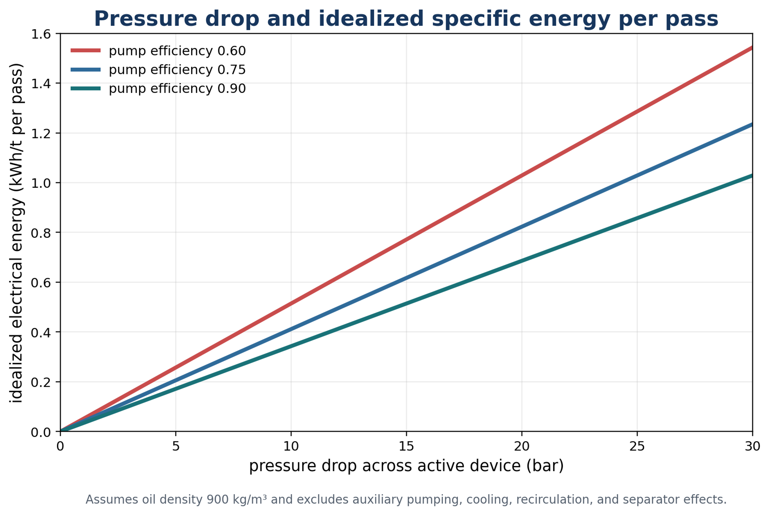
Consider 100 metric tons per hour of oil with density 900 kg per cubic meter, a device pressure drop of 15 bar, and pump efficiency 0.75. The volumetric flow is:

Hydraulic power is:

Estimated electrical power is:

The idealized specific electrical energy for one pass is:

Three equivalent passes would require about 1.85 kWh per ton before auxiliary pumps, cooling, controls, and downstream changes. This calculation does not predict process performance. It quantifies the cost of a selected pressure drop and pass count.

*Figure 8.1. Idealized pressure drop and specific electrical energy per pass for oil density of 900 kg per cubic meter at several pump efficiencies. The graph is a hydraulic calculation, not a conversion prediction [10].*

8.3 Scale up criteria

Exact geometric similarity is rarely practical because one very large throat would require extreme velocity and would not preserve turbulence structure or residence history. Industrial systems use numbering up, parallel channels, larger devices, or multiple stages. Scale up should preserve a product relevant operating window through several criteria: cavitation number, Reynolds number, pressure recovery, specific energy, temperature, residence distribution, droplet response, chemical Damkohler behavior, and separator loading [5,9].

*Figure 8.2. Scale up must preserve a product relevant operating window. Matching only pressure drop, flow, or cavitation number can fail because the other phenomena change [10].*

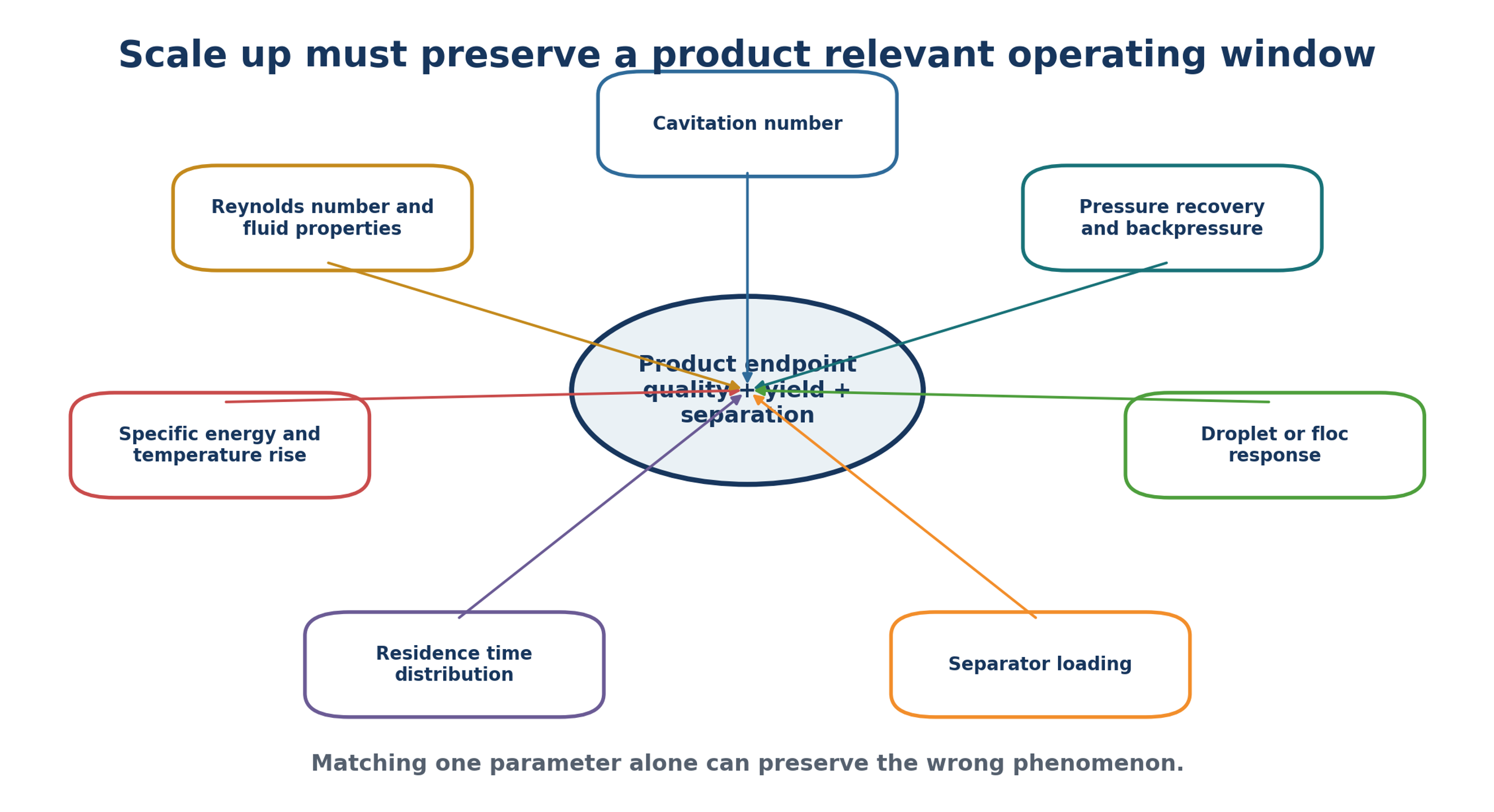
Table 8.2. Scale up criteria and verification methods.

Criterion	What should be preserved	Verification
Cavitation number	Comparable pressure and velocity relationship with same definition	Pressure and velocity at defined locations
Reynolds number	Comparable flow regime	Properties at operating temperature
Pressure recovery	Collapse location and backpressure	Axial pressure map or calibrated CFD
Specific energy	Minimum dose that reaches endpoint	Motor power per ton of on specification product
Residence distribution	Number and distribution of intense contacts and holds	Tracer testing and pass accounting
Interfacial response	Droplet or particle distribution	Laser diffraction, microscopy, or focused beam measurement
Reaction behavior	Adequate post contact reaction time	Conversion versus time and temperature
Separator load	Heavy phase flow and droplet size within capacity	Centrifuge loss, torque, and phase quality

8.4 Computational modeling

Computational fluid dynamics can compare pressure minima, vapor fraction, velocity gradients, recirculation, and likely erosion locations. Common models couple turbulence with a vapor transport equation derived from simplified bubble dynamics. The results are sensitive to nuclei assumptions, mass transfer coefficients, turbulence closure, wall roughness, and boundary pressure. A model should be calibrated against measured pressure drop, flow, temperature, vibration or acoustic response, and visualization where possible. Oil properties and dispersed phase must be represented at operating temperature. A water model can rank geometries qualitatively but can misstate absolute behavior in oil.