Hydrodynamic Cavitation Technological Equipment

5. Hydraulic and Electrical Energy

Energy accounting is often the largest source of misleading comparison among hydrodynamic cavitation studies. Hydraulic power across the cavitation device, pump shaft power, and measured electrical input are different quantities. A study that reports only ΔpQ excludes pump, motor, drive, recirculation, and auxiliary losses. A commercial process must ultimately be evaluated at the electrical or fuel meter, while the hydraulic boundary remains valuable for comparing cavitation elements independently from a particular pump [2, 3].

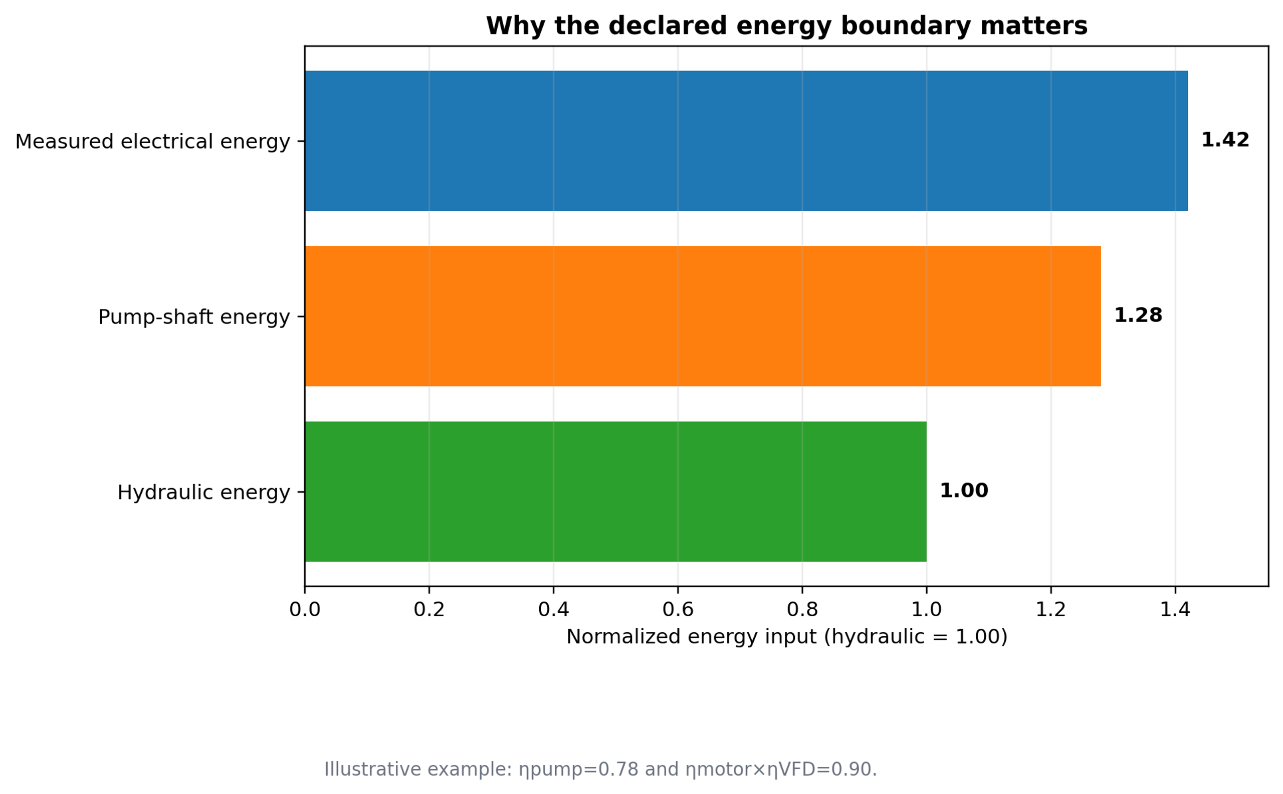
Figure 46. Why the declared energy boundary matters. The chart illustrates the same process expressed using hydraulic, shaft, and electrical input boundaries [58].

The instantaneous hydraulic power transferred across the cavitation element is:

where Δp is the defined device pressure drop and Q is volumetric flow rate. The corresponding pump shaft power is:

where ${\eta }_h$ is the pump hydraulic efficiency at the actual operating point. The electrical input is:

${\eta }_m$ and ${\eta }_{VFD}$ are motor and variable frequency drive efficiencies. The value of $P_{el}$ should be based on real electrical input at a declared boundary because motor efficiency, power factor, and drive losses change with speed and load. A noncavitating baseline can be informative, but both gross and net values should be reported.

Hydraulic and electrical energy over a test period tp are:

Integration is important when flow, pressure, or power varies during startup, batch recirculation, or temperature control. Averaging pressure and flow separately and multiplying the averages can introduce bias when the signals are correlated. A synchronized data acquisition system should therefore sample pressure, flow, power, and temperature on a common time base.

For continuous treatment, specific electrical energy consumption is:

where ṁ is mass flow rate. For a recirculated batch:

$m_b$ is processed batch mass. When the tank and external piping contain significant hold up, the denominator must include the full treated mass. SEC should be reported in J/kg, kJ/kg, kWh/t, or another clearly stated unit. Conversions between bases must not mix metric tons, short tons, and volumetric throughput.

The nominal number of passes through a recirculation loop is:

$V_b$ is the total circulating volume, including tank, piping, heat exchanger, and cavitator hold up. Equation (36) assumes perfect mixing. The actual pass distribution is broad in a stirred tank loop and may be narrower in plug flow staging. When samples are withdrawn or make up liquid is added, the calculation should be corrected by a transient mass balance.

A concentration change yield based on energy input can be defined as:

C₀ and $C_t$ are initial and final concentrations, V is treated volume, and Ein is the selected input energy. The same principle can be applied to particle size reduction, emulsification, extraction, or heating, but the numerator must be chosen before technologies are compared. For size reduction, useful metrics include change in specific surface area, log size ratio, or mass fraction below a target size. For emulsification, the full droplet size distribution and stability must accompany any single mean diameter.

If essentially all electrical energy is retained as sensible heat, the adiabatic temperature rise is:

$c_p$ is specific heat capacity. In real equipment, heat is also lost to the environment, removed by a heat exchanger, stored in metal, and carried out with product. The documented temperature rise can provide a rough energy cross check, but it does not replace the declared electrical energy basis. For deliberately heated products, the useful thermal duty should be separated from the energy associated with mixing, pumping, and pressure drop.

5.1 Complete Skid Energy and Thermal Balance

For equipment that simultaneously pumps, mixes, cavitates, and heats, the instantaneous skid boundary can be written as:

Here ${\dot{Q}}_{ret}$ is sensible or latent heat retained in the process stream, ${\dot{Q}}_{rem}$ is heat removed by a cooler, Ploss includes mechanical and environmental losses, and $dU/dt$ is energy stored in the equipment and liquid hold up. The terms are not independent during startup, when the metal and recirculation volume are warming. A steady state test should be long enough that stored energy changes are small or should explicitly integrate them over time.

When heat is an intended product of the operation, a thermal utilization ratio may be declared as:

This ratio describes energy disposition and must not be interpreted as evidence that bubble collapse creates energy. Nearly all electrical input ultimately becomes heat somewhere in the system. For a process that recovers useful heat, a net specific electrical energy can be reported separately:

The gross SEC and the recovered energy credit should both be shown. Otherwise, two studies can report the same net value while using very different pump efficiencies, cooling duties, and heat recovery assumptions. Commercial guarantees should state whether auxiliaries, recirculation, cooling, vacuum, gas compression, and cleaning energy are included.

Worked energy example. A static cavitation device operating at Q = 5 L/s and Δp = 250 kPa receives 1.25 kW of hydraulic power. With pump efficiency 0.80, motor efficiency 0.93, and drive efficiency 0.97, the estimated electrical input is about 1.74 kW. At a mass flow of 1 kg/s, the electrical SEC is about 1.74 kJ/kg, or 0.48 kWh/t. The example shows why a hydraulic only report would understate purchased energy by roughly 39%.

Table 15. Energy quantities and reporting basis.

Quantity	Boundary and method	Use	Common error
Hydraulic power, Ph	Δp across defined cavitation element multiplied by simultaneous Q	Compare device hydraulic demand	Using pump discharge pressure instead of device Δp.
Shaft power, Pshaft	Torque speed measurement or hydraulic power divided by verified pump efficiency	Pump and rotor loading	Assuming catalog efficiency at a different operating point.
Electrical power, Pel	True three phase power at motor drive input or facility meter	Purchased energy and operating cost comparison	Using voltage × current without power factor and harmonics.
Specific energy, SEC	Integrated input energy divided by actual processed mass	Compare operating conditions and technologies	Ignoring recirculation hold up or using nominal throughput.
Cavitational yield	Defined product change divided by selected energy boundary	Connect equipment input to useful result	Changing numerator or energy boundary between studies.
Thermal recovery	Heat balance over product, cooling water, metal, and losses	Separate useful heating from dissipation	Attributing all temperature rise to cavity collapse.