Hydrodynamic Cavitation in Pharmaceutical Particle Engineering, Crystallization, and Drug Delivery

2 Scientific Foundation of Hydrodynamic Cavitation and High Pressure Microchannel Processing

2.1 Hydrodynamic Cavitation Sequence

Hydrodynamic cavitation occurs when local static pressure falls to or below the effective vapor pressure of the liquid, allowing cavities to form. The cavities grow in the low pressure region and collapse when they enter a region of pressure recovery. Bubble collapse can create pressure pulses, liquid microjets, high strain rate deformation, localized energy dissipation, and steep gradients in temperature and concentration. These effects can promote particle fracture, droplet breakup, deagglomeration, surface cleaning, primary nucleation, secondary nucleation, and micromixing [1–5,29–32].

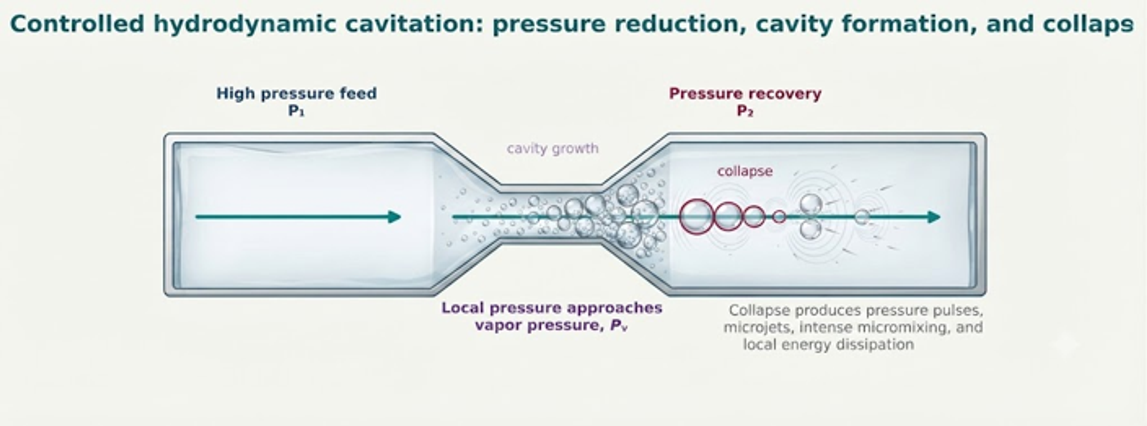
Figure 2.1. Idealized sequence of controlled hydrodynamic cavitation in a flow through constriction [42].

A convenient dimensionless indicator is the cavitation number. Definitions vary with device geometry and reference pressure, so the selected definition must be reported. Lower values generally indicate a greater tendency toward cavitation, but the cavitation number alone does not define collapse intensity or product response. Back pressure, dissolved gas, vapor pressure, temperature, viscosity, surface tension, nuclei population, residence time, and geometry remain important [1,3–5].

where σ is the cavitation number; p₂ is downstream or recovery pressure; pᵥ is liquid vapor pressure; ρ is liquid density; and u is the selected characteristic velocity.

The Reynolds and Weber numbers help separate viscous, inertial, and interfacial effects. They are especially useful when comparing devices or scaling a process across channel dimensions and flow rates. The Reynolds number characterizes the ratio of inertial forces to viscous forces:

where Re is the Reynolds number; ρ is density; u is characteristic velocity; L is characteristic length; and μ is dynamic viscosity.

The Weber number characterizes the ratio of inertial forces to interfacial (surface tension) forces:

where We is the Weber number; d is particle or droplet diameter; and γ is interfacial tension. A higher Weber number indicates greater inertial stress relative to interfacial restoring stress.

2.2 Energy Input, Dissipation, and Residence Time

Pressure alone is not a transferable measure of process severity. The specific pressure energy of an incompressible stream provides a first approximation of the maximum mechanical energy available from a pressure drop. Actual useful energy is lower because of pump losses, heat generation, flow bypass, incomplete cavitation, and energy dissipation outside the active zone.

where eₚ is the ideal specific pressure energy; Δp is pressure drop; and ρ is density.

For a defined active processing volume, mean energy dissipation rate can be estimated from power input. Local dissipation in constrictions, jets, and collapse regions can be orders of magnitude higher than the volume average. A design report should state whether the value is local, volume averaged, or system averaged.

The ideal specific pressure energy is determined by the pressure drop and fluid density:

where ε is the mean energy dissipation rate; P is power dissipated in the selected volume; ρ is density; and V is the selected active volume.

The Kolmogorov length is a turbulence scale rather than a direct particle size prediction. It indicates the smallest scale of turbulent eddies in an idealized isotropic field. When formulation structures are larger than the local dissipation scales, strong deformation and rapid micromixing become more likely. The Kolmogorov length scale is calculated from the kinematic viscosity and energy dissipation rate:

where ${\eta }_K$ is the Kolmogorov length scale; ν is kinematic viscosity; and ε is energy dissipation rate.

Residence time and exposure history are equally important. A short, intense exposure may preserve a sensitive payload better than a longer moderate exposure, even when the total energy per unit mass is similar. Recirculation creates a distribution of pass histories unless the loop volume, mixing, and withdrawal protocol are controlled.

where τ is nominal residence time; V is process or hold volume; and Q is volumetric flow rate.

2.3 Bubble Collapse Models and Their Limits

The Rayleigh collapse time provides an ideal theoretical estimate for the collapse of an empty spherical cavity in an infinite, inviscid liquid. While useful for scale reasoning, it neglects noncondensable gas, heat transfer, viscosity, compressibility, solid wall effects, neighboring cavities, and nonspherical collapse modes [2, 3]:

where $t_c$ is the ideal collapse time; R₀ is initial cavity radius; ρ is liquid density; p∞ is far field pressure; and pᵥ is vapor pressure.

The Rayleigh–Plesset equation provides a more complete radial force balance for a single spherical bubble. Although it remains an idealization when applied to dense cavity clouds, high-speed jets, or complex pharmaceutical suspensions, it rigorously clarifies how pressure, viscosity, interfacial tension, and bubble wall acceleration interact [2–5]:

where R is bubble radius; dR/dt and d²R/dt² are bubble wall velocity and acceleration; $p_B$ is pressure inside the bubble; p∞ is far field pressure; γ is surface tension; and μ is dynamic viscosity.

2.4 Microfluidizer Processing

Microfluidizer processors use a constant pressure pumping system and a fixed geometry interaction chamber. The technical documentation reports fluid velocities of up to approximately 500 m/s and identifies hydrodynamic cavitation within the interaction chambers. The principal processing mechanisms include high shear, impact against channel walls or opposing streams, turbulence within microliter volumes, and bubble collapse [17,18,33–35].

Y type chambers: These chambers are commonly promoted for oil in water emulsions, liposomes, and polymer encapsulation. The supplied documentation lists representative microchannel dimensions in the 75 to 125 µm range [33–35].

Z type chambers: These chambers are primarily used for intensive particle processing in which acceleration, turning, and impact contribute to deagglomeration and size reduction [17,18,35].

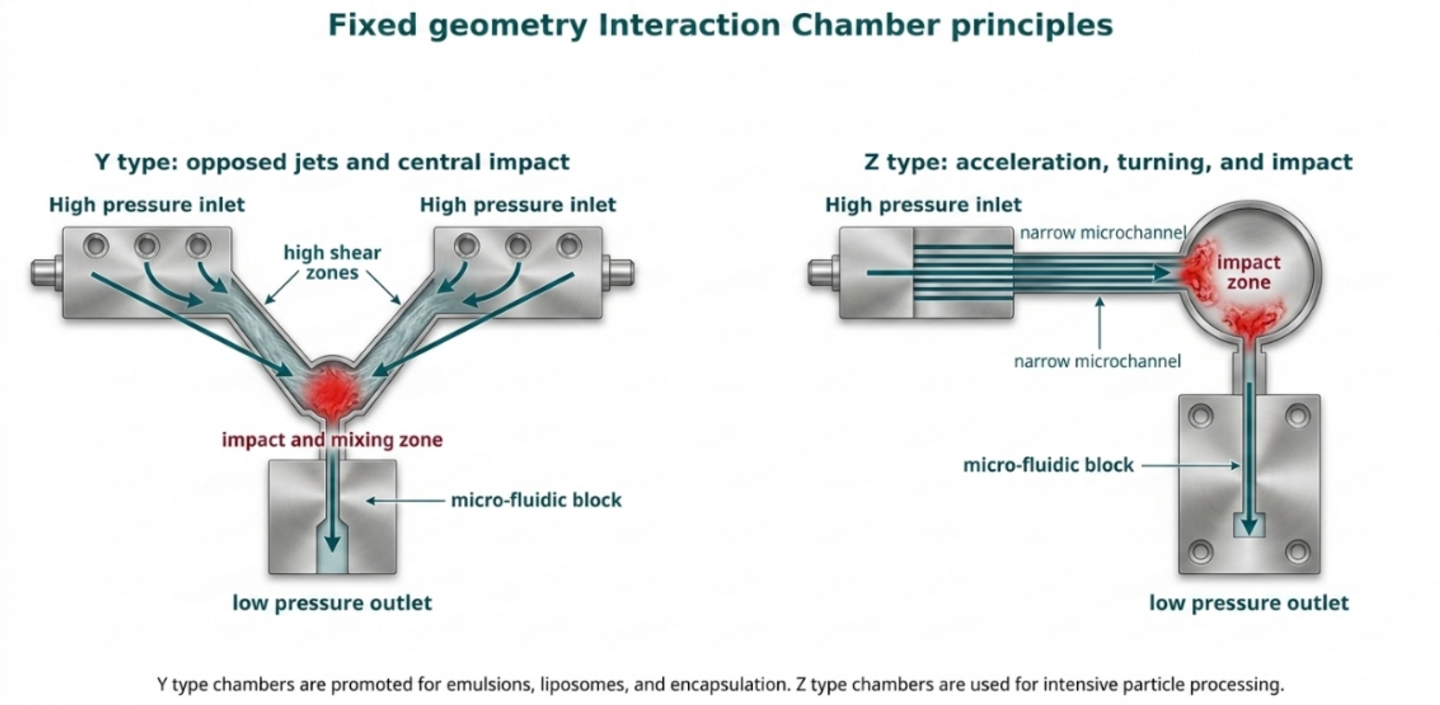
Figure 2.2. Simplified principles of Y type and Z type interaction chambers [42].