Hydrodynamic Cavitation for Wastewater Processing

8 Process Design, Scale Up, and Energy

8.1 The Operating Window

A common design error is to assume that a larger pressure drop, higher rotor speed, or lower cavitation number must monotonically improve treatment. Useful response increases after inception, reaches an operating region in which cavity population and collapse are productive, and can then decline when vapor clouds shield collapse, flow becomes choked, or energy is dissipated without sufficient chemical or biological effect. Temperature can show a similar nonmonotonic influence because increased vapor pressure promotes cavity formation while increasing vapor cushioning during collapse [1-5,16,21,30,31].

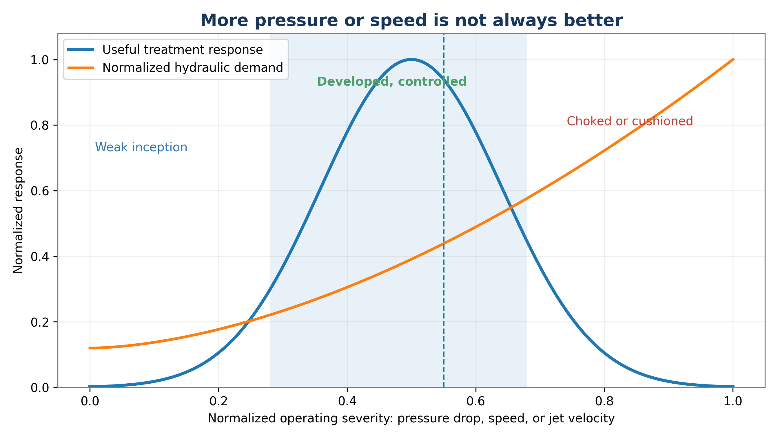
Figure 8.1. Conceptual operating window for hydrodynamic cavitation [11].

8.2 Similarity and Scale Up

Geometric similarity and a matched cavitation number do not guarantee identical treatment performance. Scale changes Reynolds number, turbulence structure, nuclei population, residence time distribution, pump efficiency, gas content, heat rejection, cavity cloud interactions, and the ratio of wall area to volume. Scale up should therefore preserve the process function, defined by the distribution of productive collapse events and the exposure of the target population or molecules.

The Reynolds number, Re, characterizes the ratio of inertial to viscous forces. The Weber number, We, characterizes the ratio of inertial to surface tension forces. A Damköhler type number, Da, compares reaction time with hydraulic exposure time. These indices supplement the cavitation number. For rotating equipment, tip speed, gap ratio, event frequency, torque, and specific power should also be considered. For jets, nozzle diameter, chamber pressure, standoff distance, entrainment, and jet interaction are important.

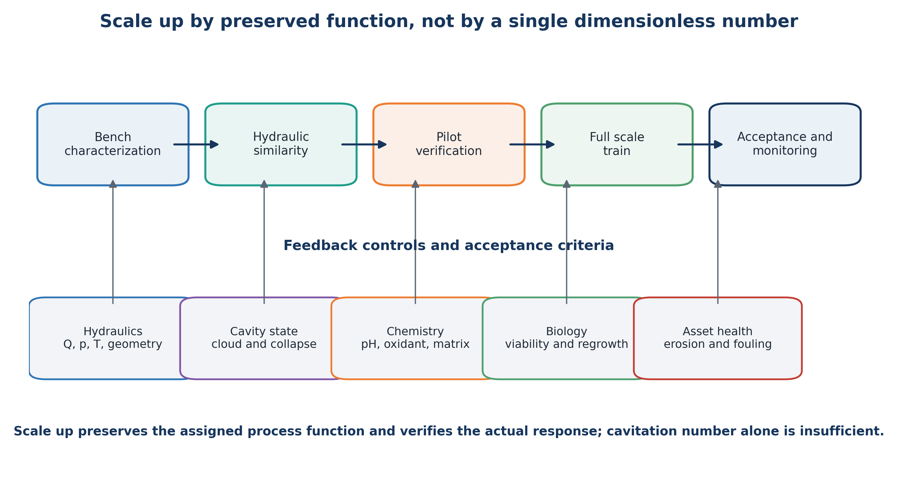
Figure 8.2. Scale up by preserving process function and verifying each development stage [11].

8.3 Energy and Economic Accounting

Energy accounting should include pumps, motors, variable frequency drives, cooling, gas compression, ozone generation, electrolysis, ultraviolet sources, plasma power, mixing, and downstream separation. Chemical production and neutralization should be included in operating cost and, when possible, in life cycle assessment. The appropriate comparison is between complete treatment trains that meet the same endpoint rather than between a cavitation pump and a single competing device [53,54].

For sludge treatment, recovered methane and reduced biosolids disposal can offset pretreatment energy. For industrial effluent, improved biological treatability can reduce aeration demand and residence time. In ballast water treatment, compactness and reduced chemical inventory can provide operational value. For micropollutants, treatment cost should be normalized to treated water volume and required removal, while recognizing that EEO does not represent toxicity or mineralization.

Table 8.1. Bench to full scale HC design checklist.

Design stage	Required evidence before proceeding
Bench characterization	Real water matrix, target endpoint, pH and temperature range, nuclei and solids behavior, oxidant demand, byproduct screen
Hydraulic development	Pressure map, flow curve, cavitation regime, heat balance, erosion location, pump efficiency, bypass and control strategy
Pilot verification	Continuous operation, residence time distribution, energy per treated volume, maintenance intervals, analytical reproducibility, toxicity and regrowth
Full scale design	Redundancy, isolation, clean in place or inspection access, replaceable wear parts, hydraulic turndown, and maintenance access
Performance verification	Performance at minimum and maximum flow, worst case water quality, defined holding time, endpoint and uncertainty, residuals, noise, and vibration
Lifecycle operation	Confirm the pressure power relation, inspect wear, update chemistry, retain treatment records, and reassess when feed composition changes

8.4 Quantitative Performance and Energy Normalization

Treatment performance should first be reported using a clearly defined analytical endpoint. For a concentration based response, percentage removal is given by:

where ηR is removal efficiency, C₀ is the initial concentration, and Ct is the concentration after treatment time t. When a pseudo first order model is justified over the measured interval, the concentration response is expressed as:

where kobs is the observed rate constant. A fitted rate constant is meaningful only when analytical method, temperature, mixing, and initial concentration are sufficiently comparable.

The hydraulic power transferred across a static cavitation device can be approximated by:

The associated electrical demand is:

where Δp is the measured pressure difference, Q is volumetric flow rate, ηp is pump efficiency, and ηm is motor and drive efficiency. For a rotating device, measured electrical or shaft power should be used directly and reported separately from auxiliary pump demand.

Specific energy input to the treated volume is:

For contaminant degradation, electrical energy per order is:

EEO is meaningful only when the same power boundary and treatment volume are used. It becomes unstable for small concentration changes and does not account for chemical consumption, cooling, or downstream process value.

A concentration based cavitational yield can be expressed as:

The nominal number of recycle turnovers and the mean hydraulic residence time are:

Nominal turnover does not imply equal exposure of every fluid element because short circuiting, dead zones, and bypass flow generate a residence time distribution. Tracer testing or computational fluid dynamics should be used when exposure uniformity is important.

Bulk temperature rise is described by the overall energy balance:

where m is liquid mass, cp is heat capacity, and Ploss is the thermal power rejected to the surroundings and cooling system. This balance separates useful thermal duty from uncontrolled heat accumulation.

For a hybrid process, a simple kinetic synergy index can be defined as:

where kHC+X is the observed rate constant for the combined process and kHC and kX are the corresponding standalone values. A value of S greater than one suggests kinetic synergy, but the conclusion should also be tested using mineralization, toxicity, and total energy and chemical cost.

A plant level net energy balance can be written as:

where recoverable biogas energy and avoided aeration or disposal energy are credited against cavitation, chemical, and cooling demands. Monetary value should be calculated separately because electricity, heat, disposal, and chemical consumption are not equivalent energy terms.

Hydraulic similarity is commonly described using the cavitation number and, for rotating equipment, rotor tip speed and power number:

Here p₂ is a downstream reference pressure, pv is vapor pressure, ρ is liquid density, vc is characteristic velocity, Dr is rotor diameter, N is rotational speed, and Pshaft is shaft power. These quantities support comparison among systems, but none uniquely determines bubble cloud structure or treatment performance. Scale up must preserve process function and verify the resulting treatment response.

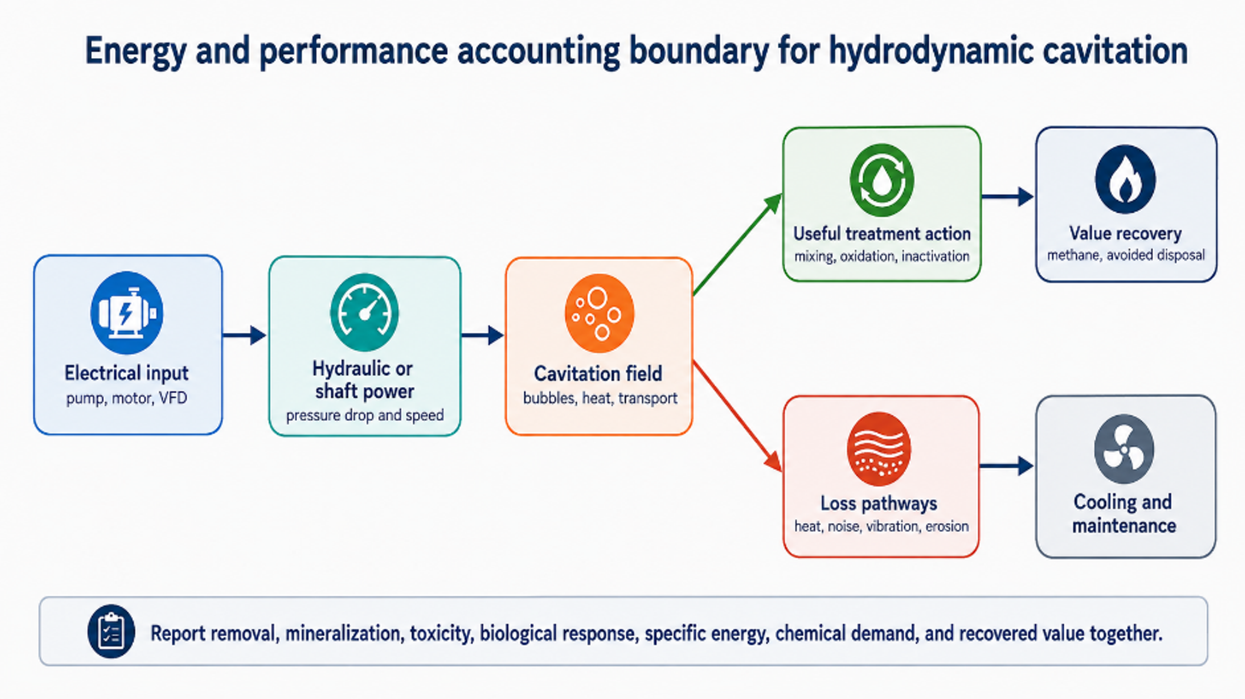
Figure 8.3. Energy and performance accounting boundary for hydrodynamic cavitation [11].

Table 8.2. Minimum normalized reporting set for HC studies and pilot trials.

Category	Minimum reported variables	Reason
Hydraulics	Flow, upstream and downstream pressure, temperature, device geometry, backpressure, loop volume, pass count	Defines the actual pressure and exposure history
Power and energy	Electrical power by component, shaft or hydraulic power, cooling duty, specific energy, EEO or yield	Prevents incomplete energy comparisons
Water matrix	pH, conductivity, alkalinity, chloride, DOC or TOC, solids, dissolved gas, initial concentration	Explains radical scavenging and cavitation changes
Treatment outcome	Parent compound, COD, TOC, biodegradability, toxicity, biological response, transformation products	Separates disappearance from useful treatment
Asset condition	Noise, vibration, erosion, fouling, pressure stability, maintenance interval	Links treatment to equipment life and operability
Uncertainty	Replicates, analytical precision, blank and thermal controls, mass balance closure	Establishes whether differences are significant

8.5 Materials, Erosion, Solids Handling, and Control

Cavitation erosion occurs when collapse is repeated on or very near a solid surface. Water treatment reactors should therefore locate the most intense collapse within the liquid whenever possible and use replaceable sacrificial components where impact cannot be avoided. Candidate materials include stainless steels, duplex alloys, hard coatings, ceramics, and engineered polymers, but selection must account for corrosion, chloride concentration, temperature, abrasive solids, cyclic stress, weld quality, and cleaning chemicals. Material ranking obtained from clean water erosion tests may change in actual wastewater.

Fibers, rags, grit, precipitates, and scale are common causes of performance loss. Upstream screening or maceration, drain and flush connections, reversible flow, accessible nozzles, and differential pressure alarms should be incorporated during initial design. Rotating equipment additionally requires seal flushing, bearing monitoring, vibration limits, and torque protection. In oxidant systems, compatible seals and controlled injection location are required to prevent concentrated chemical attack.

A robust control system maintains the desired operating window rather than a fixed pump pressure alone. Manipulated variables may include motor speed, control valve position, downstream backpressure, recycle ratio, gas injection, oxidant dose, and cooling flow. Protective interlocks should respond to low flow, excessive temperature, pressure instability, vibration, seal failure, high residual oxidant, and loss of neutralization capacity.

Table 8.3. Common failure modes and engineering safeguards.

Failure mode	Likely cause	Process consequence	Safeguard or diagnostic
Loss of cavitation response	Nozzle wear, blockage, gas change, backpressure drift	Lower oxidation, lysis, or inactivation	Pressure profile, acoustic or vibration signature, power and flow trend
Excessive vapor structure	Backpressure too low or temperature too high	Vapor shielding and weak collapse	Control downstream pressure and temperature
Rapid erosion	Collapse attached to wall, abrasive solids, unsuitable material	Metal loss, contamination, unplanned outage	Move collapse zone, replaceable insert, erosion inspection coupon
Plugging or ragging	Fibers, grit, precipitate, inadequate screening	Flow imbalance and pump overload	Macerator, screen, flush ports, differential pressure alarm
Biological deterioration after sludge treatment	Excessive exposure or inhibitory soluble products	Lower methane yield or unstable digestion	BMP testing, staged treated fraction, SCOD and ammonia monitoring
Oxidant inefficiency	Overdose, scavenging, poor injection, incorrect pH	Higher chemical cost and byproducts	Dose response testing, residual measurement, TOC and toxicity
Uncontrolled heating	High recirculation power and insufficient cooling	Confounded kinetics, vapor pressure change, safety risk	Heat balance, cooling loop, temperature interlock

8.6 Pilot Protocol and Acceptance Criteria

Pilot development should proceed through defined evidence gates. The first stage maps clean water hydraulics and identifies stable ranges of pressure, flow, temperature, power, vibration, and backpressure. The second stage uses a safe tracer or model target to confirm residence time distribution and analytical repeatability. The third stage treats actual wastewater across the expected seasonal matrix range. The final stage operates continuously for sufficient duration to reveal fouling, erosion, sensor drift, maintenance demand, and downstream biological response.

Acceptance criteria must be linked to the plant objective. A polishing system may be evaluated using micropollutant removal, toxicity, and EEO. A sludge system requires net methane production, solids reduction, dewatering performance, and digester stability. A ballast water system requires certified biological performance and residual control. A precipitation system requires dissolved nutrient or metal removal together with acceptable solids separation. In every case, the guaranteed operating boundary should define feed quality, flow rate, temperature, and required auxiliary chemicals.

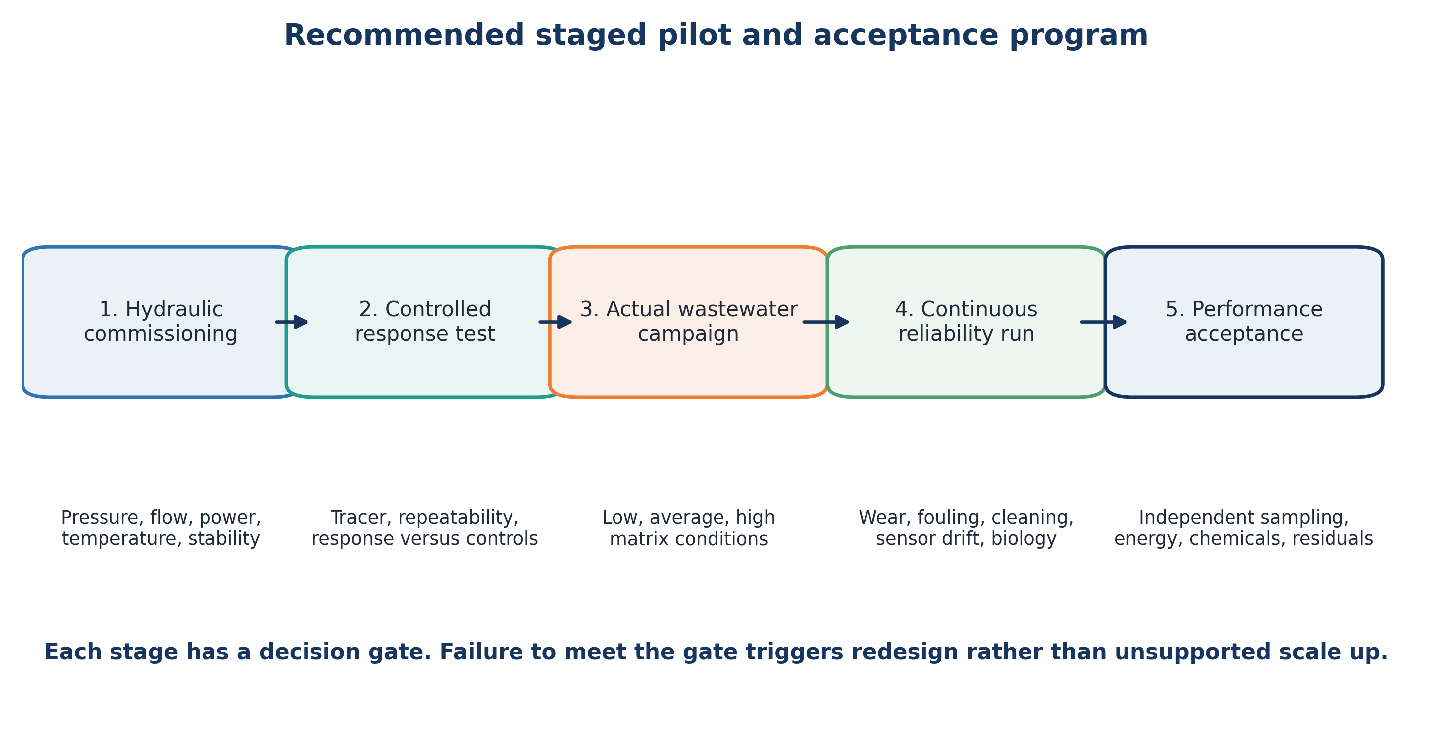
Figure 8.4. Recommended staged pilot and acceptance program [11].

Table 8.4. Recommended staged pilot program.

Stage	Feed and duration	Primary measurements	Decision gate
1. Hydraulic commissioning	Clean water over full pressure and flow map	Pressure profile, flow, power, temperature, vibration, cavitation stability	Safe and repeatable operating envelope
2. Controlled response	Model solute, tracer, or standardized sludge test	Residence time distribution, removal kinetics, heat balance, replicate uncertainty	Evidence that response tracks controllable variables
3. Actual wastewater campaign	Representative low, average, and high load matrices	Target removal, TOC or COD, toxicity, SCOD or BMP, chemical demand	Site specific optimum and treatment train position
4. Continuous reliability run	Weeks to months at design duty	Wear, fouling, cleaning, sensor drift, availability, downstream process impact	Maintainable design and realistic operating cost
5. Performance acceptance	Contract feed window and independent sampling	Guaranteed endpoints, energy, chemicals, residuals, asset condition	Documented compliance and handover criteria