# Cavitation Driven Exfoliation of Graphene and Two Dimensional Materials
## Abstract
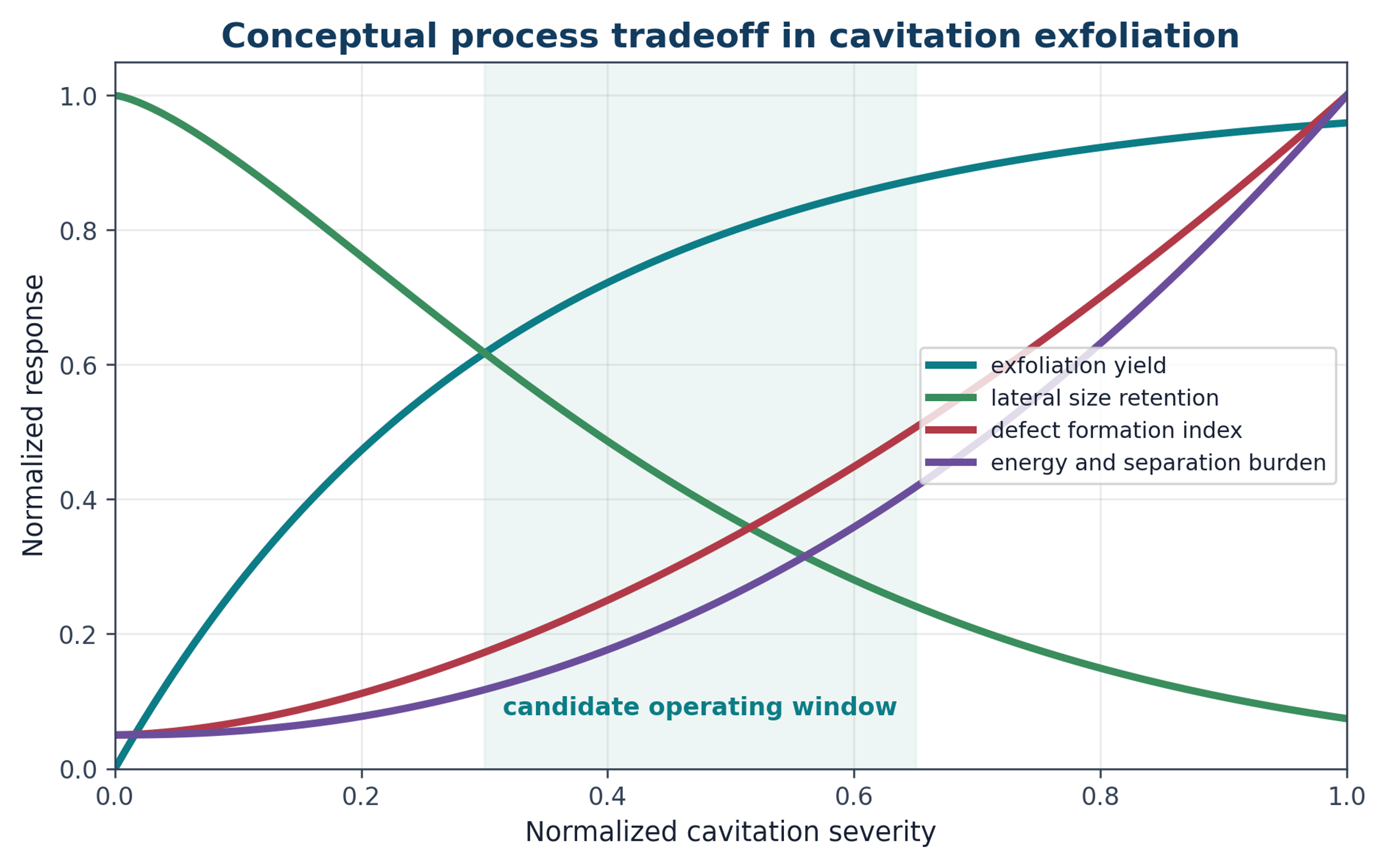
Cavitation assisted liquid phase exfoliation provides a scalable top down route for producing graphene and other two dimensional materials without necessarily relying on strong oxidative chemistry. This article examines the thermodynamic basis of layer separation, liquid wetting and stabilization, cavitation physics, stress transfer to layered particles, and the operating characteristics of acoustic and hydrodynamic reactors. Jet cavitation, microfluidic cavitation, rapid decompression, microfluidization, wet jet milling, rotor stator processing, and hybrid routes are evaluated together with downstream classification, concentration, drying, formulation, and quality assurance. Published evidence shows that useful exfoliation requires a controlled balance between delamination and damage. Increasing treatment severity can reduce thickness but can also decrease lateral size, increase edge density and basal plane defects, generate holes, accelerate stabilizer degradation, increase equipment wear, and reduce isolated yield. Product quality therefore cannot be defined by a single metric. Raman spectroscopy, AFM, TEM, surface chemistry, trace contamination, dispersion stability, mass balance, and application performance must be interpreted together. Scale up should preserve effective exposure, pressure recovery, residence time distribution, solids loading, thermal history, and classification conditions rather than equipment size or nominal power alone. The same framework extends to boron nitride, transition metal dichalcogenides, black phosphorus, layered oxides, MXenes, and clays. Cavitation is most effective when it is integrated into specification driven manufacturing and evaluated by reproducible mass of in specification product per unit time, energy, and process burden.
## 1 Introduction
This article establishes a common engineering framework for hydraulic definitions, energy boundaries, residence time, uncertainty, and scale translation, and then applies that framework to cavitation driven exfoliation of graphene and related two dimensional materials.
The isolation of graphene demonstrated that a stable sheet only one atom thick can be separated from a bulk layered crystal while retaining exceptional electronic, thermal, optical, and mechanical properties [1]. This achievement also defined a manufacturing challenge. Methods that produce ideal flakes for laboratory study do not necessarily provide the mass throughput, consistency, cost, or formulation behavior required for industrial use. Graphene manufacturing therefore spans a broad product range, from isolated monolayers to few layer graphene, graphene nanoplatelets, expanded graphite, functionalized graphene related materials, and application specific masterbatches.
The term graphene must be used precisely. ISO terminology distinguishes graphene from bilayer graphene, few layer materials, graphene nanoplatelets, graphene oxide, reduced graphene oxide, and other two dimensional materials [3]. These distinctions are technically significant because layer number, flake thickness, lateral dimension, disorder, surface chemistry, impurity content, aggregation state, and specific surface area determine suitability for inks, polymer composites, cement, lubricants, thermal interfaces, battery electrodes, catalyst supports, membranes, and sensors. Structural characterization therefore treats thickness, lateral size, disorder, layer alignment, and specific surface area as separate measurands [4]. Chemical characterization additionally includes elemental composition, oxygen to carbon ratio, trace metals, and functional group analysis [5].
Liquid phase exfoliation is attractive because a layered solid can be separated in a liquid without necessarily requiring strong oxidation. The liquid wets newly created surfaces, transmits mechanical stress, suppresses direct particle contact, and can serve as the final formulation medium. Cavitation based exfoliation is one branch of this approach. Vapor or gas cavities form, grow, and collapse, generating pressure pulses, shock waves, microjets, turbulent shear, particle collisions, and rapid pressure release. These events can overcome interlayer attraction and generate nanosheets, but they can also cut flakes, create edge defects, damage basal planes, erode equipment, heat the liquid, and degrade stabilizers. Process design must therefore balance delamination against structural damage [7-13,17].
Graphene is used as the principal case study because the cavitation literature is most extensive for this material. The same engineering framework is then extended to hexagonal boron nitride, molybdenum disulfide, tungsten disulfide, black phosphorus, layered oxides, MXenes, and layered silicates. The objective is not to identify a universally superior reactor, but to establish a framework for selecting, measuring, scaling, and controlling a process against a defined product specification.
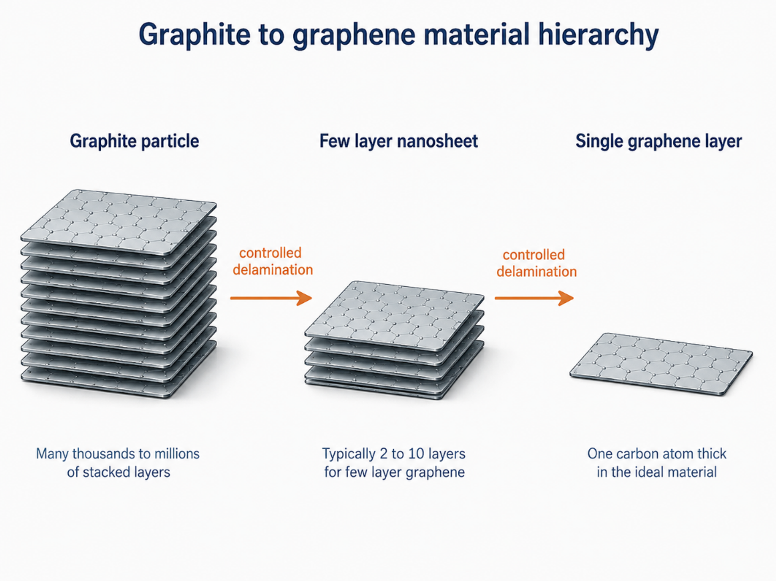
Figure 1.1. Hierarchy from a graphite particle to a few layer nanosheet and an ideal single graphene layer. Industrial powders normally contain a distribution rather than one uniform layer count [37]Source citation in original document: [37].
*[Figure 1.1](#figure-1-1). Hierarchy from a graphite particle to a few layer nanosheet and an ideal single graphene layer. Industrial powders normally contain a distribution rather than one uniform layer count [37].*
## 2 Scope, Terminology, and Product Classes
A production route should begin with a written material specification rather than with the unrestricted goal of making graphene. The specification should define the intended product form, such as powder, concentrated paste, aqueous dispersion, organic dispersion, polymer masterbatch, conductive ink, or directly compounded composite. It should also define acceptable distributions of layer number, thickness, lateral size, oxygen content, trace metal content, residual stabilizer, moisture, ash, and agglomerate size. ISO/TS 9651:2025 provides a classification framework intended to improve consistency in commercial descriptions [6].
*Table 2.1. Working terminology for graphene related products used in this article [3-6].*
| **Term** | **Practical description** | **Critical measurements** | **Typical processing relevance** |
|------------------------------------------|---------------------------------------------------------------------------------------------------------------|-----------------------------------------------------------------------------------|------------------------------------------------------------------------------------------------|
| Graphene | A single carbon layer in a hexagonal lattice. | AFM or TEM thickness, Raman 2D band, defects, contamination. | Research and high value electronic or sensing applications. |
| Bilayer graphene | Two well defined graphene layers. | Layer count, stacking, lateral size, Raman peak shape. | Electronic, optical, and model material studies. |
| Few layer graphene | A small number of graphene layers, commonly treated as three to ten in industrial discussion. | Thickness distribution, Raman response, edge and basal plane defects. | Inks, composites, coatings, energy storage, and thermal products. |
| Graphene nanoplatelets | Platelet shaped graphene related particles with nanometre scale thickness and much larger lateral dimensions. | Thickness, aspect ratio, specific surface area, oxygen, ash, residual graphite. | High volume composite, construction, lubricant, and barrier applications. |
| Graphene oxide | Oxidized graphene related sheets with oxygen containing functionality. | Oxygen to carbon ratio, functional groups, layer size, residual salts and metals. | Water dispersions, membranes, functional materials. It is not equivalent to pristine graphene. |
| Reduced graphene oxide | Partly deoxygenated graphene oxide. | Residual oxygen, lattice disorder, conductivity, impurity content. | Conductive and electrochemical products where perfect lattice restoration is not required. |
| Graphite nanosheets or expanded graphite | Thin graphitic particles that remain thicker than few layer graphene. | Thickness, expansion ratio, particle size distribution, accessible surface area. | Useful intermediate or final additive when full exfoliation is unnecessary. |
> ***Note. The exact product designation should be linked to measured ranges and the intended application. A single average value can conceal a broad distribution that is commercially and technically important.***
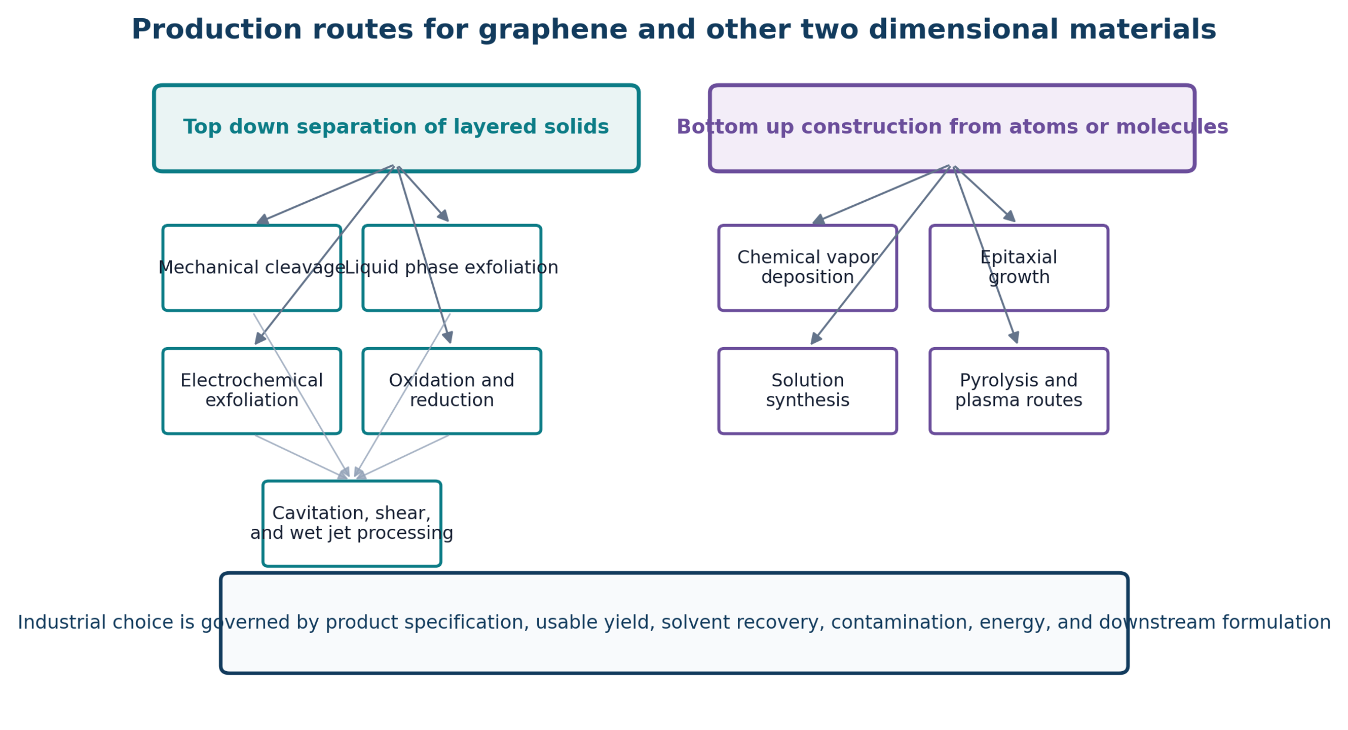
Figure 2.1. Major top down and bottom up routes for graphene and other two dimensional materials. Cavitation belongs to top down liquid processing and frequently operates together with shear, collision, pressure release, and classification [37]Source citation in original document: [37].
*[Figure 2.1](#figure-2-1). Major top down and bottom up routes for graphene and other two dimensional materials. Cavitation belongs to top down liquid processing and frequently operates together with shear, collision, pressure release, and classification [37].*
## 3 Structure, Interlayer Attraction, and Exfoliation Thermodynamics
### 3.1 Layered Crystal Geometry
Graphite consists of graphene layers bonded strongly within each basal plane and held together much more weakly between planes. The large difference between in plane bonding and interlayer attraction permits sliding and peeling. Similar structural anisotropy occurs in many layered solids, although the interlayer interaction may include van der Waals attraction, electrostatic contributions, ionic character, surface oxidation, adsorbed water, or intercalated species. Consequently, identical reactor settings can produce substantially different outcomes for graphite, boron nitride, transition metal dichalcogenides, black phosphorus, and layered oxides.
The ideal minimum work required to create two new surfaces can be represented by a surface energy balance. For flake area A and effective cleavage energy Gc, the reversible work is:
(3.1)
Wmin is the ideal minimum work, Gc is the effective cleavage energy per unit area, and A is the newly separated area. Actual process energy is substantially greater because only a fraction of the supplied energy is transmitted to an advancing interlayer crack.
The engineering objective is not simply to exceed the ideal cleavage work. Stress must be transmitted to a defect, edge, fold, gallery, or liquid wedge in a direction that advances separation. Energy dissipated as uniform heating, pumping loss outside the active region, or random turbulence remote from particles does not directly create product. Nominal motor power is therefore an inadequate basis for comparison unless calorimetry, hydraulic power, active volume, residence time, and recovered product mass are also reported.
### 3.2 Wetting and Solvent Matching
Freshly separated surfaces tend to restack unless the liquid and any stabilizer reduce the free energy of dispersion. Solvent screening can use surface tension, solubility parameters, polarity, hydrogen bonding capability, viscosity, boiling point, toxicity, cost, and recoverability. Mixtures can be more effective than a single liquid because they allow surface energy and viscosity to be adjusted independently. A hydrodynamic study using isopropyl alcohol and water found an optimum near 40 volume percent isopropyl alcohol, where surface tension, Hansen distance, viscosity, and dispersion stability provided a favorable combination [15]. To quantify thermodynamic affinity and compatibility between a solid solute or nanoparticle () and the liquid solvent medium (), the Hansen solubility parameter distance () is used Equation (3.2):
(3.2)
Ra is the Hansen solubility parameter distance between solid s and liquid l. δD, δP, and δH are dispersive, polar, and hydrogen bonding components. While a smaller value generally indicates higher thermodynamic compatibility and wetting propensity between the liquid and the solid surface, solubility parameters alone are insufficient for dynamic systems. Effective process optimization requires simultaneously accounting for hydrodynamic constraints, such as cavitation bubble dynamics, liquid compressibility, and medium viscosity.
Surfactants and polymers can adsorb on newly exposed surfaces and provide electrostatic, steric, or combined stabilization. Sodium cholate, sodium deoxycholate, carboxymethyl cellulose, polyvinylpyrrolidone, proteins, and other dispersants have been used. Stabilizer concentration should be optimized rather than maximized. Insufficient stabilizer permits restacking, whereas excessive stabilizer increases viscosity, foaming, purification burden, conductivity loss, and cost. Cavitation can also degrade the stabilizer, so stability must be measured after processing rather than inferred from the initial formulation [10-14,20,21].
*Table 3.1. Selection factors for the liquid medium and stabilizer.*
| **Factor** | **Why it matters** | **Preferred evidence** | **Common failure mode** |
|-----------------------------|------------------------------------------------------------------------------------------|--------------------------------------------------------------------------------------------------------------------|------------------------------------------------------------------------------------------------------|
| Surface compatibility | Controls wetting, dispersion free energy, and restacking tendency. | Measured concentration after standardized separation; long term sedimentation; Hansen or surface energy screening. | A liquid that wets graphite initially but cannot stabilize the thinner product. |
| Viscosity | Affects shear stress, pressure loss, cavitation inception, heat generation, and pumping. | Viscosity at process temperature and solids loading. | A formulation that cavitates well when dilute but becomes noncavitating at production concentration. |
| Vapor pressure | Changes bubble formation and collapse intensity. | Vapor pressure and cavitation number at actual temperature. | Excessive vapor cushioning or insufficient cavity formation. |
| Boiling point and recovery | Determines drying duty, solvent loss, and residual solvent. | Mass balance around recovery equipment and residual solvent analysis. | High energy drying or unsafe vapor accumulation. |
| Stabilizer adsorption | Prevents restacking and controls rheology. | Zeta potential, rheology, TGA, surface analysis, redispersion test. | Excess residue lowers electrical or thermal performance. |
| Corrosion and compatibility | Protects pumps, seals, valves, nozzles, and analytical equipment. | Materials compatibility test and extractables analysis. | Metal contamination or seal swelling. |
| Safety and environment | Determines containment, ventilation, fire protection, and waste treatment. | SDS, exposure assessment, flash point, emissions and waste inventory. | A laboratory solvent that is unacceptable at plant scale. |
## 4 Cavitation Physics and Force Transmission
### 4.1 Pressure Reduction and Cavitation Number
Hydrodynamic cavitation begins when local static pressure approaches the liquid vapor pressure or when dissolved gas and heterogeneous nuclei expand under reduced pressure. A simplified Bernoulli relation illustrates the coupling among static pressure, velocity, and elevation:
(4.1)
p is static pressure, ρ is liquid density, u is mean velocity, g is gravitational acceleration, z is elevation, and hL represents irreversible head loss. While rigorous modeling of real cavitating flows requires advanced two-phase Eulerian-Eulerian or mixture frameworks coupled with turbulence closures, simplified scaling parameters remain invaluable for preliminary design intuition. The intensity of cavitation is primarily governed by the dimensionless cavitation number ():
(4.2)
σ is the cavitation number, is a reference upstream or local pressure, is vapor pressure, ρ is density, and u is the selected reference velocity. Lower σ generally indicates stronger cavitation, but geometry and nuclei distribution affect the observed regime.
A constriction does more than reduce pressure. It accelerates particles, generates high velocity gradients, changes platelet orientation, creates turbulent eddies, and can focus collisions at walls or channel junctions. The pressure recovery zone determines where bubbles collapse. Collapse within a controlled chamber can transfer useful mechanical energy to particles, whereas collapse in a pump, valve seat, or downstream pipe primarily promotes erosion rather than exfoliation.
### 4.2 Bubble Dynamics
The radial behavior of an isolated spherical bubble in an infinite liquid is commonly represented by the Rayleigh-Plesset equation. Although this relation does not fully describe a bubble cloud adjacent to a flake, it identifies the principal roles of pressure, density, viscosity, surface tension, gas content, and time:
(4.3)
R is bubble radius, Ṙ and R¨ are radial velocity and acceleration, pB is pressure inside the bubble, p∞ is far field pressure, μ is dynamic viscosity, γ is surface tension, and ρ is liquid density.
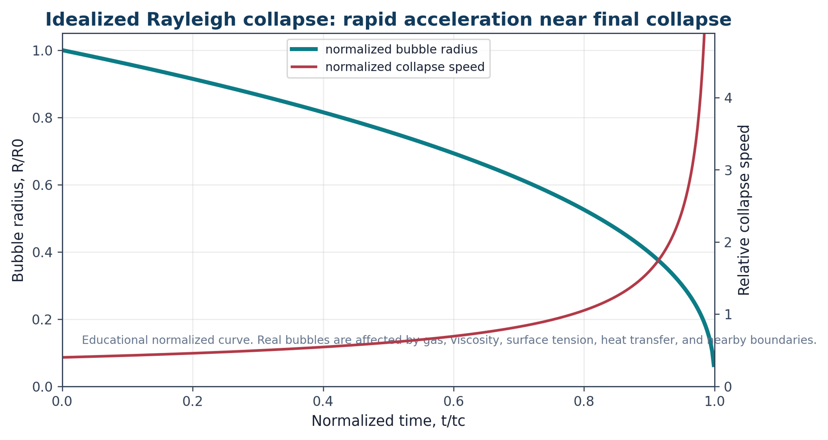
Figure 4.1. Normalized educational representation of rapid bubble collapse. Collapse velocity increases strongly near the final stage, which helps explain intense local pressure pulses [37]Source citation in original document: [37].
*[Figure 4.1](#figure-4-1). Normalized educational representation of rapid bubble collapse. Collapse velocity increases strongly near the final stage, which helps explain intense local pressure pulses [37].*
Practical exfoliation occurs within bubble clouds, near solid surfaces, and in particle laden flow. Synchronized collapse of a bubble cloud can produce a pressure pulse greater than that associated with an isolated bubble. High speed and X-ray free electron laser imaging reported in [17] showed that quasi simultaneous cloud collapse can generate shock waves that interact with two dimensional materials on nanosecond time scales. These observations support both immediate fracture and fatigue accumulated through repeated pressure pulses.
### 4.3 Stress Pathways in Layered Particles
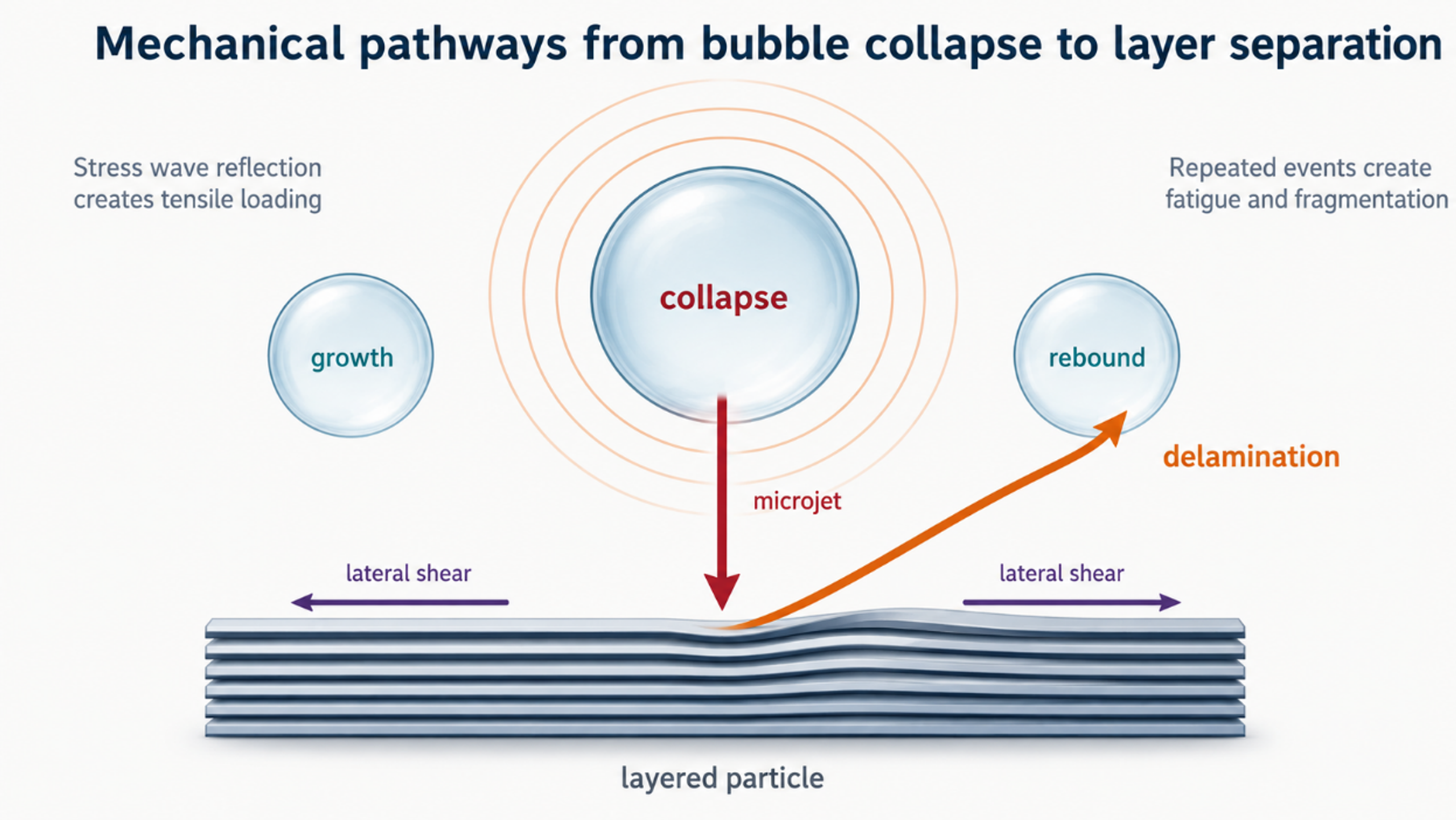
Several mechanical pathways operate simultaneously. A compressive wave entering a particle can reflect from a particle liquid interface as a tensile wave and promote separation. A bubble collapsing near a surface can form an asymmetric microjet. Velocity gradients impose viscous shear, turbulent fluctuations impose Reynolds stress, and particle collisions or wall impacts introduce bending and edge damage. Pressure retained within defects or liquid filled galleries can be released when the surrounding pressure decreases. Repeated pulses can extend cracks even when an individual event remains below the threshold for complete separation [7-12,17]. The characteristic shear rate is determined by the velocity difference across a gap or boundary layer and the effective gap thickness:
(4.4)
γ̇ is a characteristic shear rate, Δu is the velocity difference across a gap or boundary layer, and is the effective gap thickness. The viscous shear stress () for a Newtonian approximation is given by:
(4.5)
τ is viscous shear stress for a Newtonian approximation. Concentrated graphite dispersions may be non-Newtonian, so apparent viscosity at the process shear rate should be used.
(4.6)
Re is Reynolds number and Dh is hydraulic diameter. In particle laden and cavitating flow this value is a scaling indicator, not a complete description of turbulence or two phase structure.
Figure 4.2. Mechanical pathways by which bubble collapse, pressure waves, microjets, lateral shear, and repeated fatigue can separate or fragment layered particles [7-12,17]Source citations in original document: [7-12,17].
*[Figure 4.2](#figure-4-2). Mechanical pathways by which bubble collapse, pressure waves, microjets, lateral shear, and repeated fatigue can separate or fragment layered particles [7-12,17].*
*Table 4.1. Mechanisms contributing to cavitation assisted exfoliation.*
| **Mechanism** | **Primary loading direction** | **Useful effect** | **Possible damage or limitation** |
|-------------------------------|-------------------------------------------------|----------------------------------------------------------|--------------------------------------------------------------------------------|
| Stress wave reflection | Normal to the basal plane or particle surface. | Opens preexisting cracks and separates adjacent layers. | Can fracture brittle flakes or create holes when impulse is excessive. |
| Microjet impact | Localized normal and tangential loading. | Initiates peeling at edges, folds, or surface defects. | Highly localized damage and equipment erosion. |
| Viscous shear | Parallel to adjacent layers. | Promotes interlayer sliding and continuous delamination. | Cuts large flakes when stress or exposure is excessive. |
| Turbulent Reynolds stress | Fluctuating lateral and normal loading. | Repeated random loading over the particle population. | Broad product distribution when residence time is broad. |
| Particle collision | Impact, bending, and edge loading. | Creates fresh edges and assists self-exfoliation. | Introduces fragmentation, contamination, and abrasion. |
| Pressure release in galleries | Normal expansion from internal liquid or gas. | Can open intercalated or defect rich structures. | Requires wetting and may produce uncontrolled expansion. |
| Fatigue from repeated passes | Repeated subcritical normal and lateral stress. | Raises exfoliation fraction without one extreme event. | Defect accumulation, heating, stabilizer degradation, and diminishing returns. |
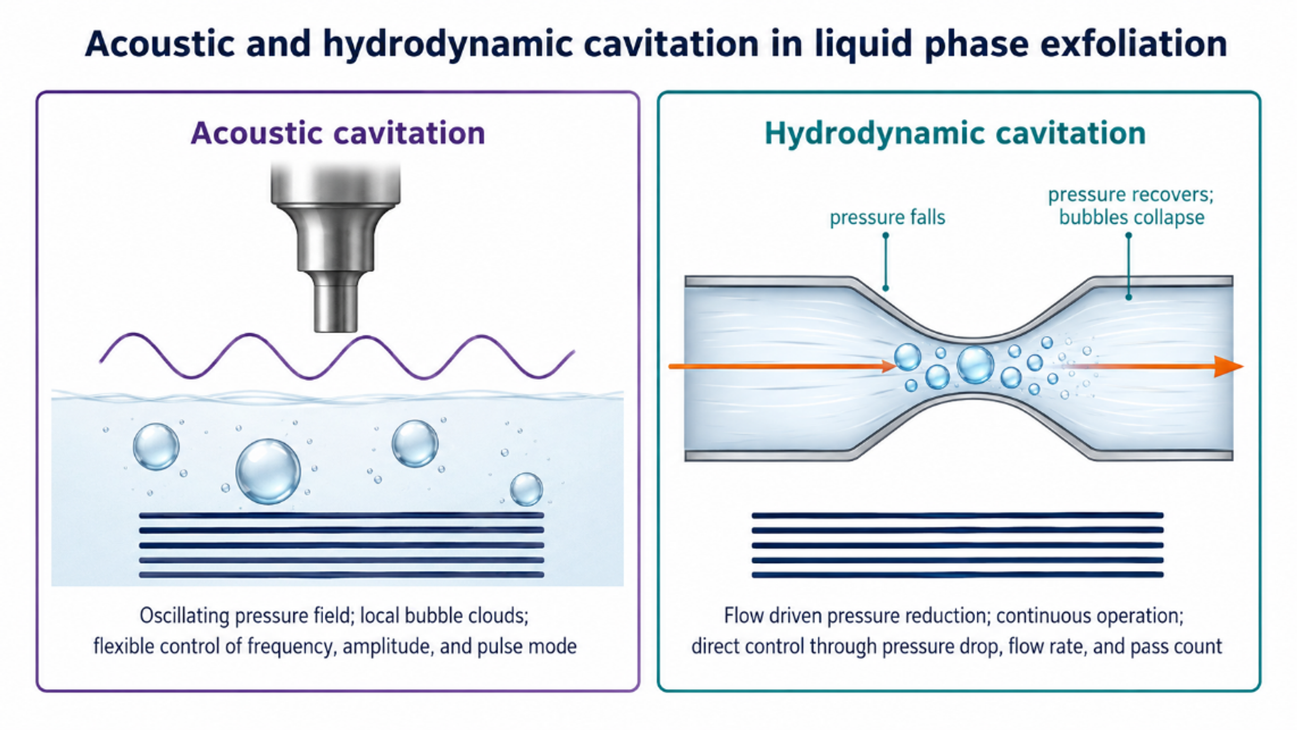
Figure 4.3. Comparison of acoustic and hydrodynamic cavitation fields. Both create bubbles and collapse events, but the field geometry, residence time, and scale up variables differ [37]Source citation in original document: [37].
*[Figure 4.3](#figure-4-3). Comparison of acoustic and hydrodynamic cavitation fields. Both create bubbles and collapse events, but the field geometry, residence time, and scale up variables differ [37].*
## 5 Acoustic Cavitation Exfoliation
### 5.1 Reactor Types and Operating Variables
Acoustic cavitation uses alternating pressure generated by an ultrasonic bath, probe, horn, sonotrode, plate transducer, focused source, or flow cell. Frequencies near 20 to 40 kHz commonly generate strong inertial cavitation and comparatively large transient bubbles, whereas higher frequencies can produce smaller bubbles and a more distributed field. Frequency alone does not define process severity. Amplitude, transducer area, immersion depth, pulse mode, static pressure, liquid temperature, gas content, vessel geometry, solids loading, and acoustic attenuation all influence the active bubble population.
Bath sonication is convenient for screening but often transfers only a small and poorly quantified fraction of electrical power to the sample. Probe systems provide much greater local intensity, but exposure can be highly nonuniform. Material near the probe tip can experience severe cavitation, heating, and sonotrode erosion while the remainder of the vessel receives lower intensity. Flow cells, multiple transducers, and pressurized reactors improve control by defining the treated volume and residence time.
(5.1)
Iac is nominal acoustic intensity, Pac is acoustic power delivered to the liquid, and Atr is active transducer area. The value should be based on measured or calorimetric power, not only the electrical nameplate.
(5.2)
Pcal is calorimetric power, is liquid mass, cp is heat capacity, and dT/dt is the initial temperature rise rate under insulated or corrected conditions.
The in situ imaging study reported in [17] is important because it shifts interpretation from a qualitative hot spot concept toward measurable shock wave and bubble cloud dynamics. It also supports the practical observation that controlled pulsing, pressure, and circulation can improve acoustic processing by reducing shielding and distributing cavitation events more uniformly.
*Table 5.1. Key variables for acoustic exfoliation experiments and scale up.*
| **Variable** | **Recommended report** | **Reason** | **Control action** |
|--------------------------|-------------------------------------------------------------------|-----------------------------------------------------------------------|------------------------------------------------------------------------------------------|
| Frequency | Fundamental and any secondary frequency, kHz or MHz | Changes bubble size, threshold, and spatial distribution. | Select single or multiple frequency operation for target thickness and defect tolerance. |
| Delivered power | Calorimetric power and power density. | Electrical input does not equal power in the liquid. | Calibrate each vessel and fill level. |
| Amplitude and pulse mode | Tip amplitude, duty cycle, pulse duration. | Controls peak pressure and thermal accumulation. | Use pulse sequences to limit shielding and heating. |
| Static pressure | Absolute vessel pressure and gas condition. | Changes cavitation threshold and collapse intensity. | Use controlled back pressure where equipment permits. |
| Temperature | Continuous liquid temperature, not only initial value. | Changes viscosity, vapor pressure, gas solubility, and stabilization. | Provide cooling and define a temperature window. |
| Geometry | Tip diameter, immersion depth, vessel dimensions, flow cell path. | Determines field uniformity and inactive zones. | Use mapping, dosimetry, or acoustic emission monitoring. |
| Exposure | Residence time distribution, recirculation flow, and passes. | Average time can hide overtreated and undertreated fractions. | Prefer controlled flow exposure for scale up. |
### 5.2 Product Quality and Limits
Acoustic treatment can produce monolayer and few layer material, but the measured product distribution depends strongly on post processing. Centrifugation commonly removes unexfoliated graphite and sorts material by sedimentation behavior. Reported yield therefore depends on the centrifugation protocol, collected fraction, extinction coefficient used for concentration, and whether yield refers to monolayers, material below a thickness threshold, or all solids retained in the supernatant. A meaningful comparison must state the yield definition explicitly.
Ultrasonic power exhibits an optimum rather than an unlimited benefit. In MoS₂ exfoliation, concentration increased with power and then declined at excessive intensity because cavitation shielding altered the effective field. Flake size also responded nonmonotonically [18]. The same principle applies to graphite. Excessive severity can increase fragmentation faster than useful delamination and can produce a stable dispersion of small defective fragments that appears optically dark but does not meet the intended product specification.
## 6 Hydrodynamic Cavitation Exfoliation
### 6.1 Devices and Flow Regimes
Hydrodynamic cavitation can be generated by flow through a constriction, Venturi throat, orifice, nozzle, valve, rotor stator gap, interaction chamber, microchannel, or wet jet processor. The method is naturally compatible with continuous pumping and recycle. The active field can be described by pressure drop, flow rate, back pressure, geometry, cavitation number, residence time, and pass count. These variables are generally more directly scalable than nominal ultrasonic amplitude, although the flow remains complex and equipment wear can be substantial.
The hydraulic power made available across a pressure reduction element is:
(6.1)
Ph is pump shaft power required for the useful pressure drop, Δp is pressure difference, Q is volumetric flow rate, and ηp is overall pump efficiency. The actual system power also includes recirculation, cooling, mixing, and separation.
(6.2)
Ev is the ideal cumulative hydraulic energy density for Np identical passes when each pass dissipates approximately Δp joules per cubic meter. This relation is a first order accounting tool and does not identify the fraction coupled to exfoliation*.*
(6.3)
is specific process energy per mass of recovered product, t is processing time, and is recovered product mass. This metric exposes low usable yield that can be hidden by energy per liter.
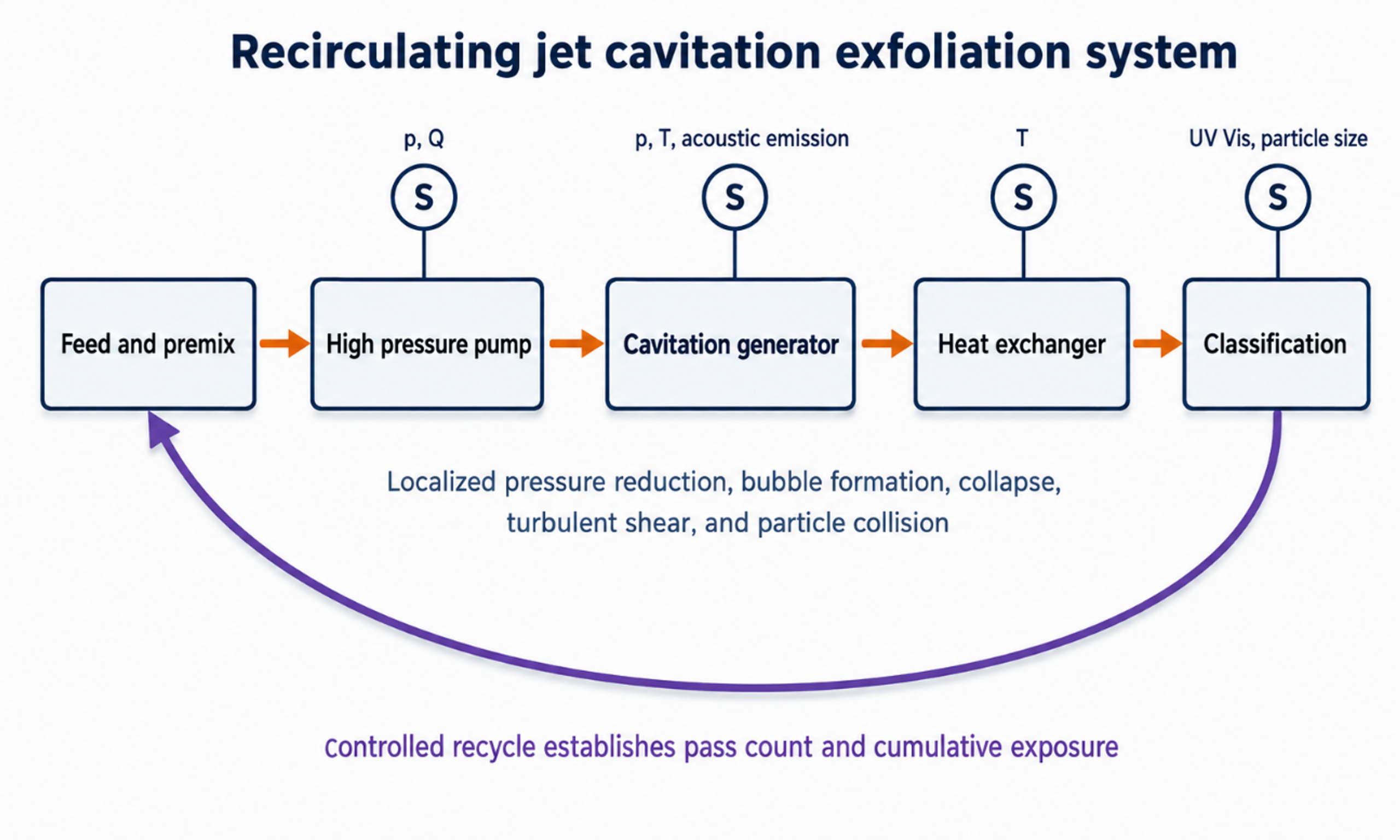
Figure 6.1. Recirculating jet cavitation system with pressure, flow, temperature, acoustic emission, and product sensors. Controlled recycle establishes cumulative exposure [37]Source citation in original document: [37].
*[Figure 6.1](#figure-6-1). Recirculating jet cavitation system with pressure, flow, temperature, acoustic emission, and product sensors. Controlled recycle establishes cumulative exposure [37].*
### 6.2 Jet Cavitation Evidence
One of the earliest jet cavitation demonstrations processed a 30 kg aqueous suspension containing 1.9 mass percent crystalline graphite, 0.1 mass percent carboxymethyl cellulose, and 98 mass percent water at 20 MPa for 30 min. AFM, TEM, and Raman analyses supported the presence of monolayer and few layer material, with an estimated total graphene yield near 4 mass percent [7,8]. The study established process feasibility and proposed a mechanical mechanism based on stress wave reflection at the graphite liquid interface.
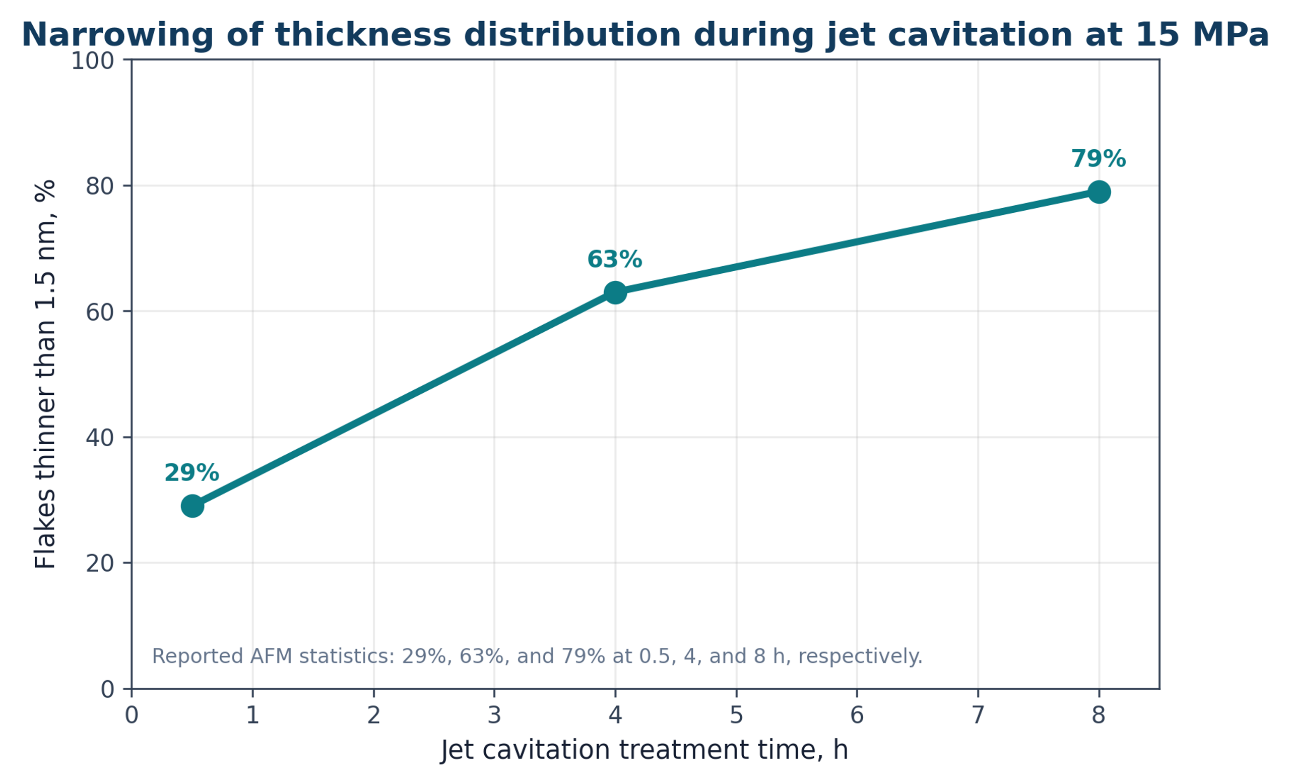
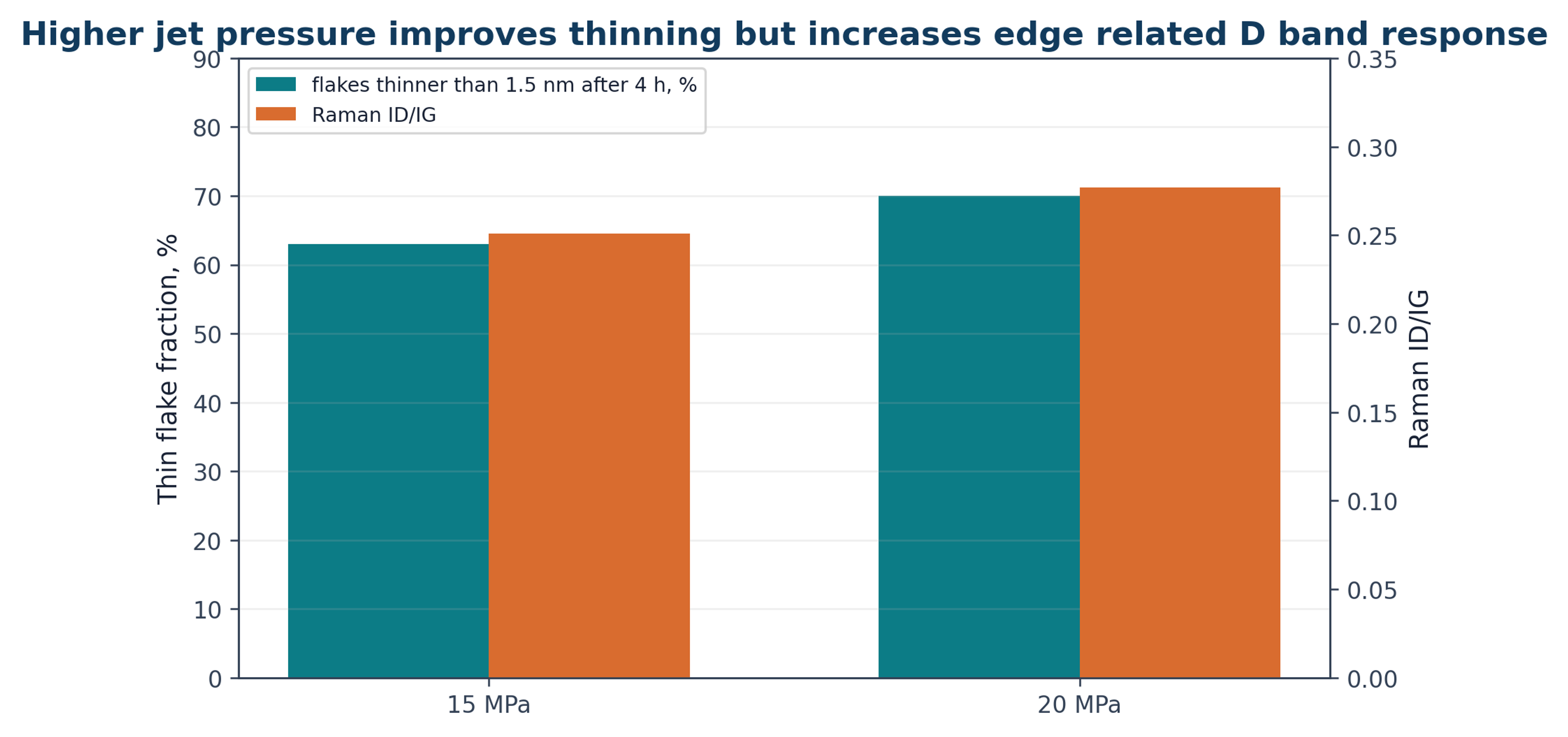
A later parameter study used a 10 L graphite dispersion in an acetone water mixture. At an initial graphite concentration of 1 mg mL⁻¹, 20 MPa, and 8 h, the reported exfoliation fraction reached approximately 12 mass percent. At 15 MPa, the fraction of flakes thinner than 1.5 nm increased from 29 percent after 0.5 h to 63 percent after 4 h and 79 percent after 8 h. Increasing pressure to 20 MPa increased the thin flake fraction but also raised Raman ID/IG from approximately 0.251 to 0.277, consistent with greater edge generation [9].
Figure 6.2. Reported increase in the fraction of flakes thinner than 1.5 nm with jet cavitation treatment time at 15 MPa [9]Source citation in original document: [9].
*[Figure 6.2](#figure-6-2). Reported increase in the fraction of flakes thinner than 1.5 nm with jet cavitation treatment time at 15 MPa [9].*
Figure 6.3. Pressure related tradeoff between thinning and Raman D band response. The 20 MPa condition produced a larger thin flake fraction and a slightly larger ID/IG ratio [9]Source citation in original document: [9].
*[Figure 6.3](#figure-6-3). Pressure related tradeoff between thinning and Raman D band response. The 20 MPa condition produced a larger thin flake fraction and a slightly larger ID/IG ratio [9].*
The concentration study also showed that increasing graphite loading does not necessarily increase graphene output. At high initial loading, the product concentration plateaued and could decrease. Particle loading changes turbulence, bubble nucleation, viscosity, collision frequency, and access to the active region. Scale up should therefore consider the coupled relationship among solids loading, active flow volume, pressure drop, residence time, and heat removal rather than feed concentration alone.
### 6.3 Hydrodynamic Cavitation on a Chip
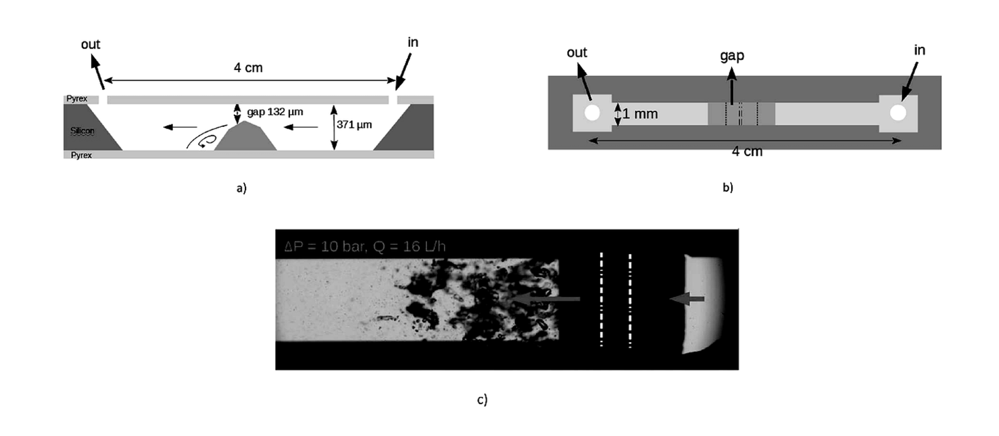
Microfluidic cavitation devices provide well defined geometry and permit direct visualization of the flow field. Qiu and coauthors used a silicon and glass device with a 132 micrometer gap, a 10 bar pressure drop, and a flow rate of 16 L h⁻¹. A 50 g L⁻¹ graphite suspension stabilized with 1 g L⁻¹ sodium cholate received approximately 2000 passes. Characterization showed monolayer and few layer graphene with lateral dimensions of several hundred nanometers [10]. The device required modest hydraulic power, but throughput and clogging remain important scale up constraints.
Figure 6.4. Profile view, top view, and cavitating flow image for the hydrocavitating lab on a chip used by Qiu and coauthors. The local step creates a low pressure recirculation region followed by bubble collapse [10]Source citation in original document: [10]. License stated in bibliography: CC BY NC 3.0.
*[Figure 6.4](#figure-6-4). Profile view, top view, and cavitating flow image for the hydrocavitating lab on a chip used by Qiu and coauthors. The local step creates a low pressure recirculation region followed by bubble collapse [10].*
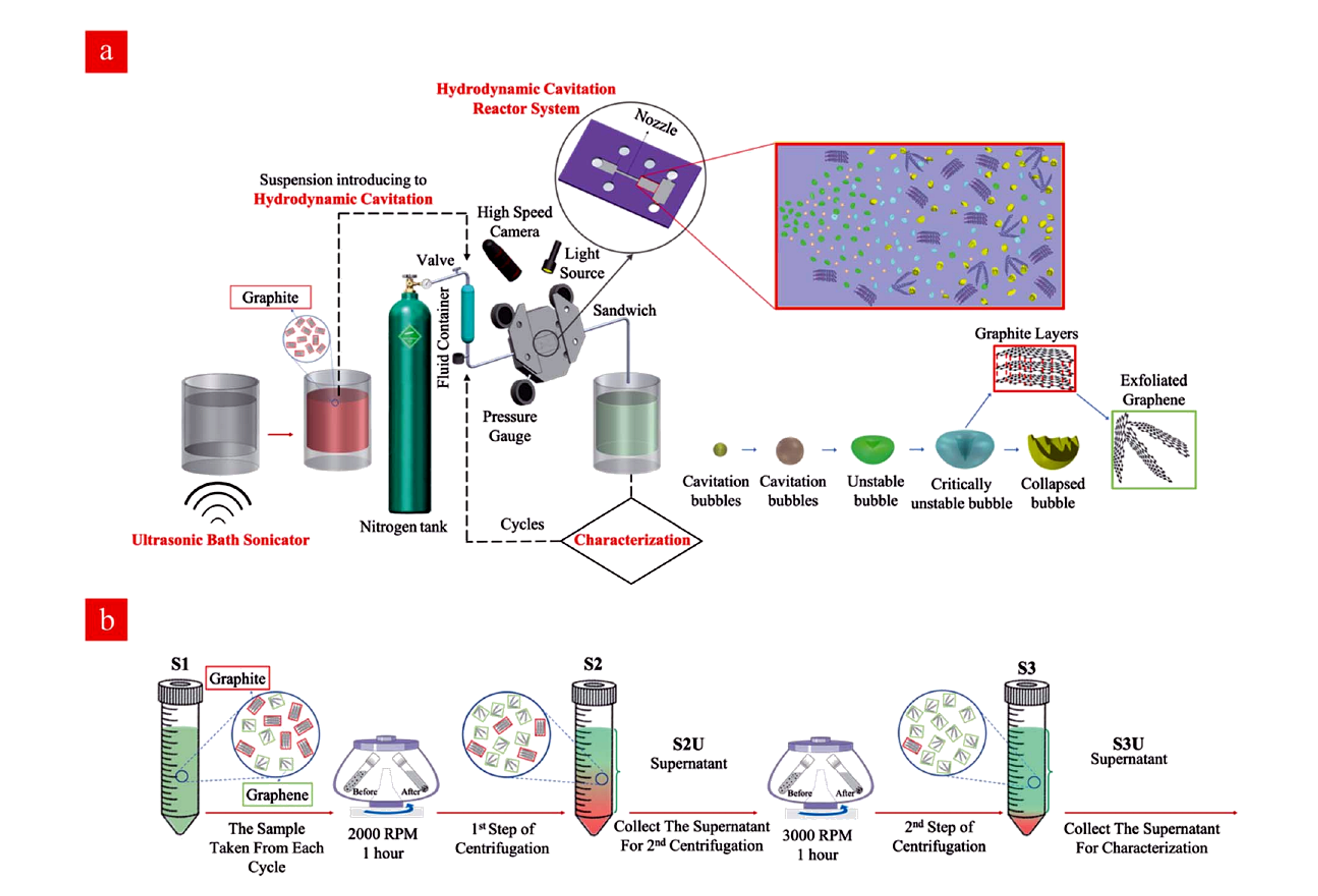
Jafarpour and coauthors used a pressure resistant microreactor containing an inlet, nozzle, extension section, and engineered roughness. Natural graphite was processed in water without a surfactant, and 650 psi was selected for repeated treatment. Cavitation inception decreased from approximately 220 psi on the first cycle to about 140 psi after 80 cycles, while a fully developed pattern appeared near 300 psi after extensive cycling. The authors attributed this shift to an increasing population of heterogeneous nuclei as particles became smaller and more numerous [11].
Figure 6.5. Hydrodynamic cavitation reactor system and sequential centrifugation workflow used for water based graphene nanosheet preparation [11]Source citation in original document: [11]. License stated in bibliography: CC BY 3.0.
*[Figure 6.5](#figure-6-5). Hydrodynamic cavitation reactor system and sequential centrifugation workflow used for water based graphene nanosheet preparation [11].*
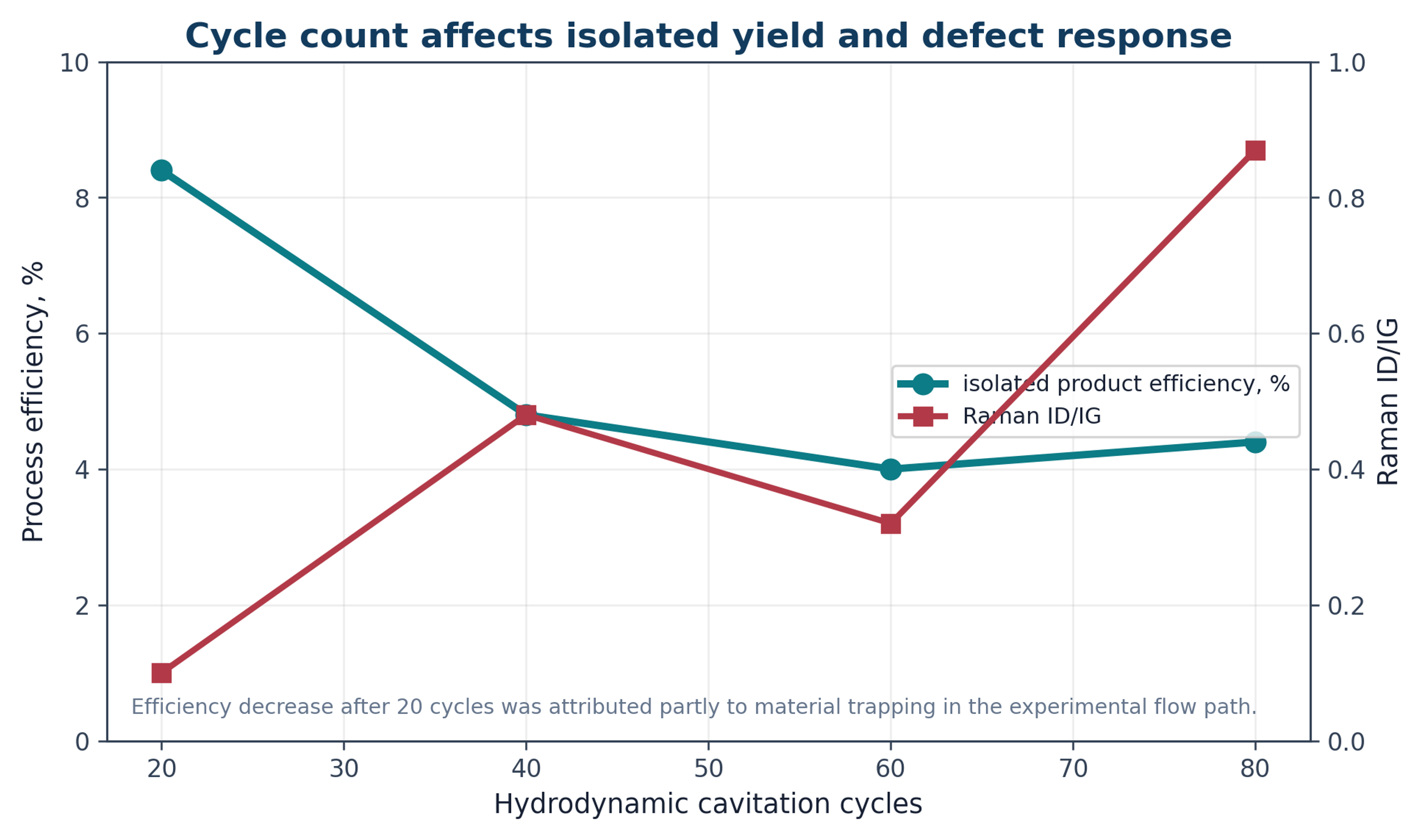
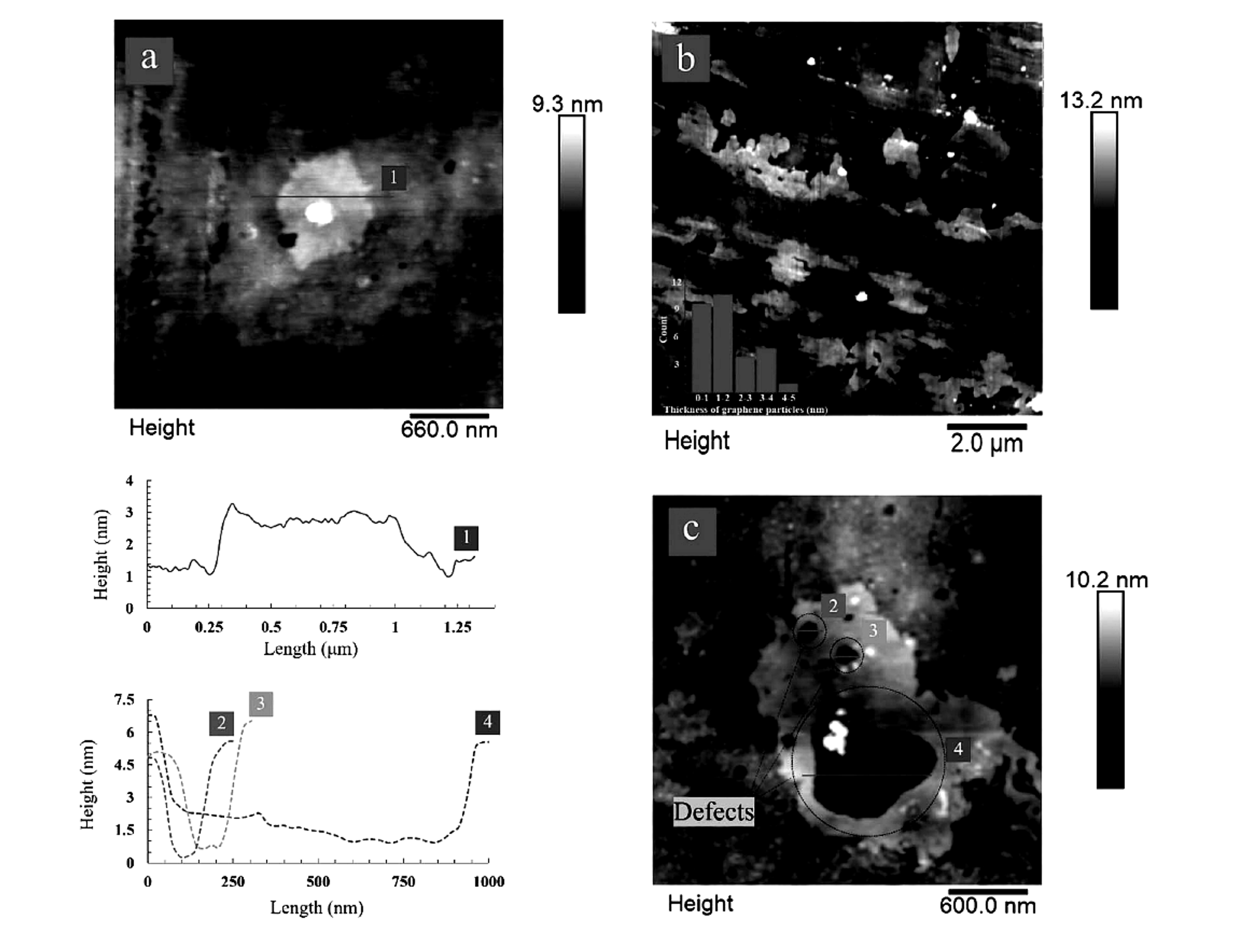
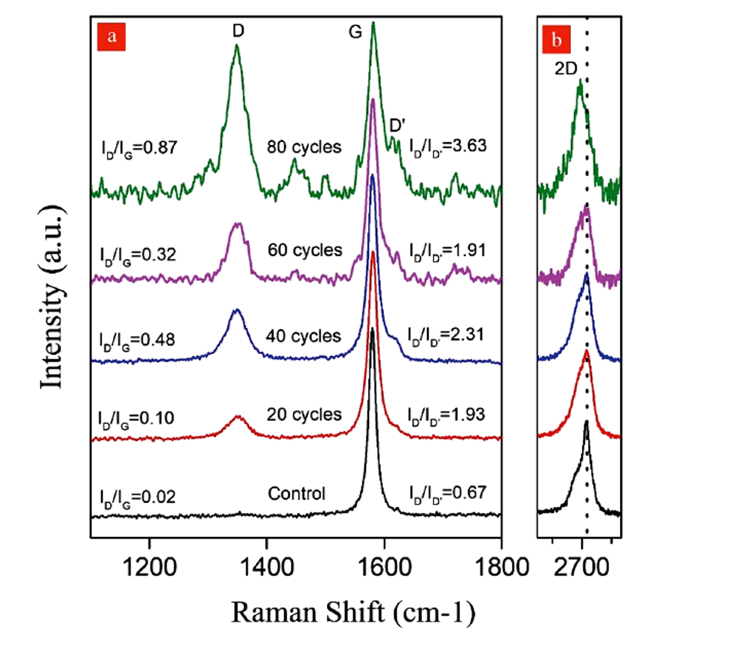
AFM showed material approximately 1 nm thick after 80 cycles and a thickness range of 1.2 to 2.5 nm after 60 cycles, with lateral dimensions of approximately 1 to 5 micrometers. Excessive exposure generated holes about 100 to 600 nm across. Isolated product efficiencies after 20, 40, 60, and 80 cycles were reported as 8.4, 4.8, 4.0, and 4.4 percent, respectively. The decrease after the first sampling point was attributed partly to material trapping in the experimental flow path, illustrating that system holdup can distort an apparent yield trend [11].
Figure 6.6. Effect of hydrodynamic cavitation cycle count on isolated product efficiency and Raman ID/IG in the microreactor study [11]Source citation in original document: [11]. License stated in bibliography: CC BY 3.0.
*[Figure 6.6](#figure-6-6). Effect of hydrodynamic cavitation cycle count on isolated product efficiency and Raman ID/IG in the microreactor study [11].*
Figure 6.7. AFM images and height profiles showing thin graphene sheets and cavitation induced defects after repeated cycles [11]Source citation in original document: [11]. License stated in bibliography: CC BY 3.0.
*[Figure 6.7](#figure-6-7). AFM images and height profiles showing thin graphene sheets and cavitation induced defects after repeated cycles [11].*
### 6.4 Protein Stabilized Hydrodynamic Exfoliation
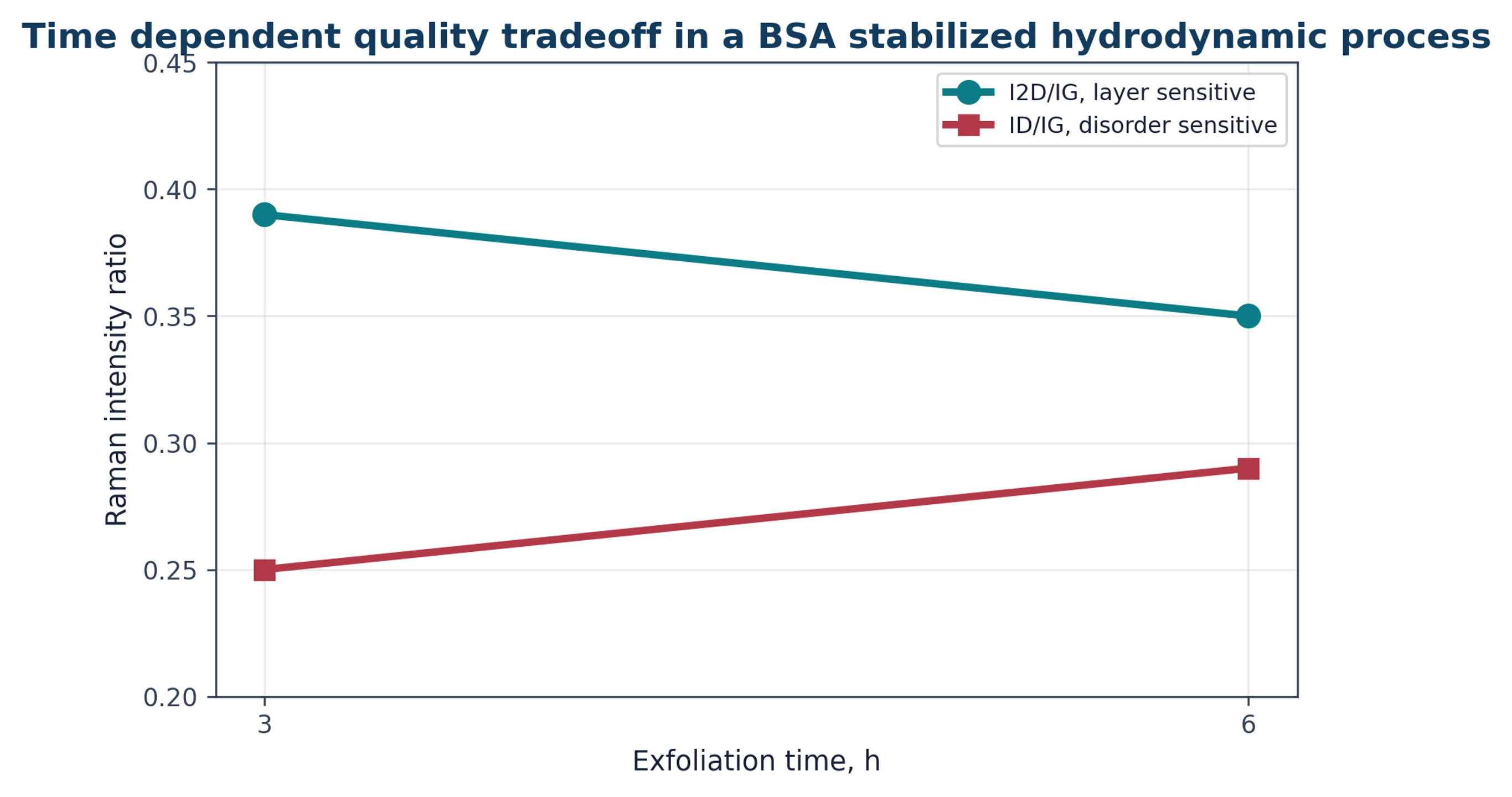
A hydrodynamic process using bovine serum albumin as an exfoliation and stabilization agent illustrates the competition among product quality indicators. At 3 h, I2D/IG was reported as 0.39 and ID/IG as 0.25. At 6 h, I2D/IG decreased to 0.35 while ID/IG increased to 0.29. The trend indicates continued evolution of layer structure together with increasing disorder. Protein stabilization may be useful for biological formulations, but the protein becomes part of the product and may be unacceptable for electronic, thermal, or high temperature applications [12].
Figure 6.8. Time dependent Raman ratios in a bovine serum albumin stabilized hydrodynamic cavitation process [12]Source citation in original document: [12].
*[Figure 6.8](#figure-6-8). Time dependent Raman ratios in a bovine serum albumin stabilized hydrodynamic cavitation process [12].*
## 7 Rapid Decompression, Waterjet, and Patent Defined Architectures
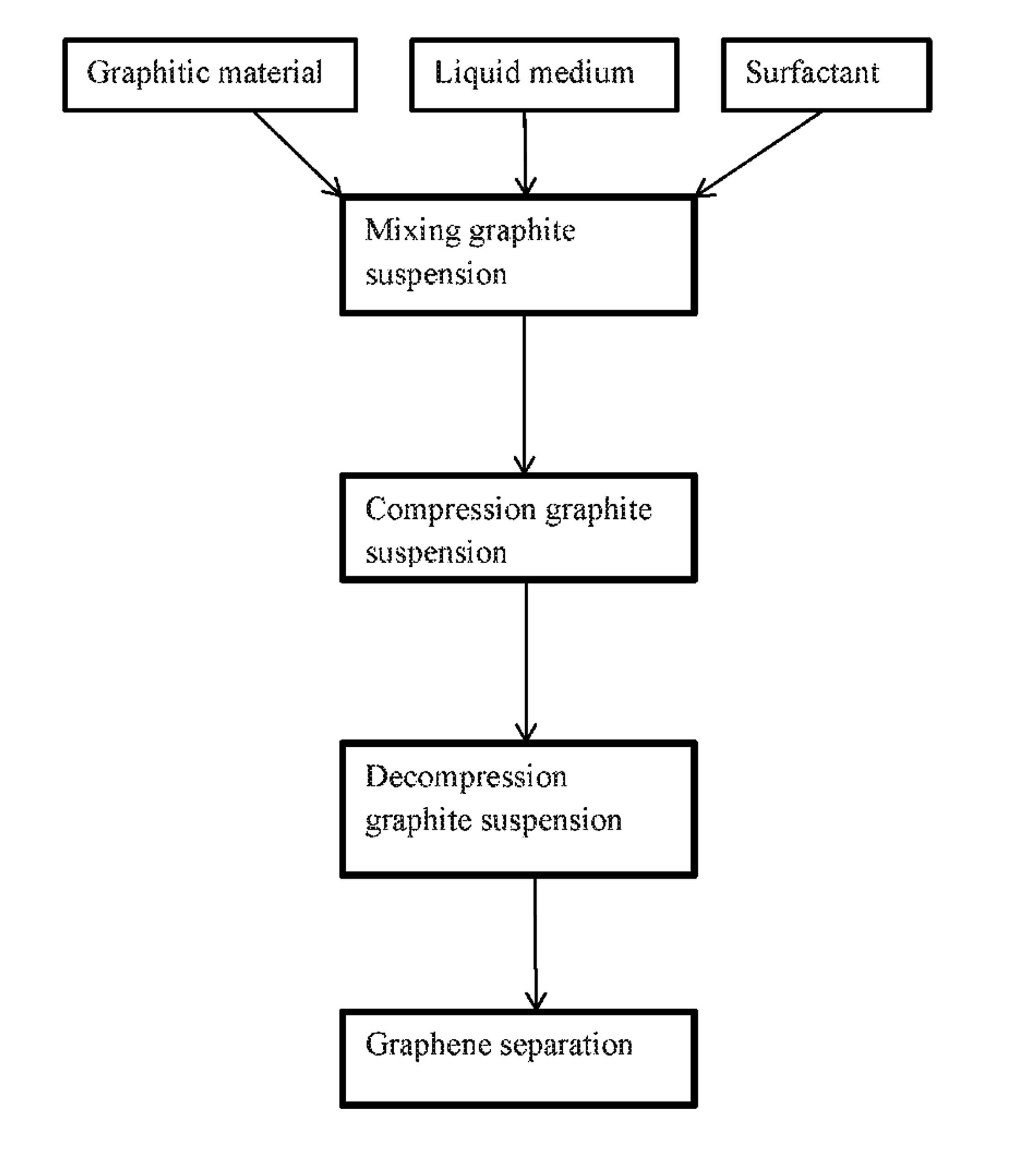
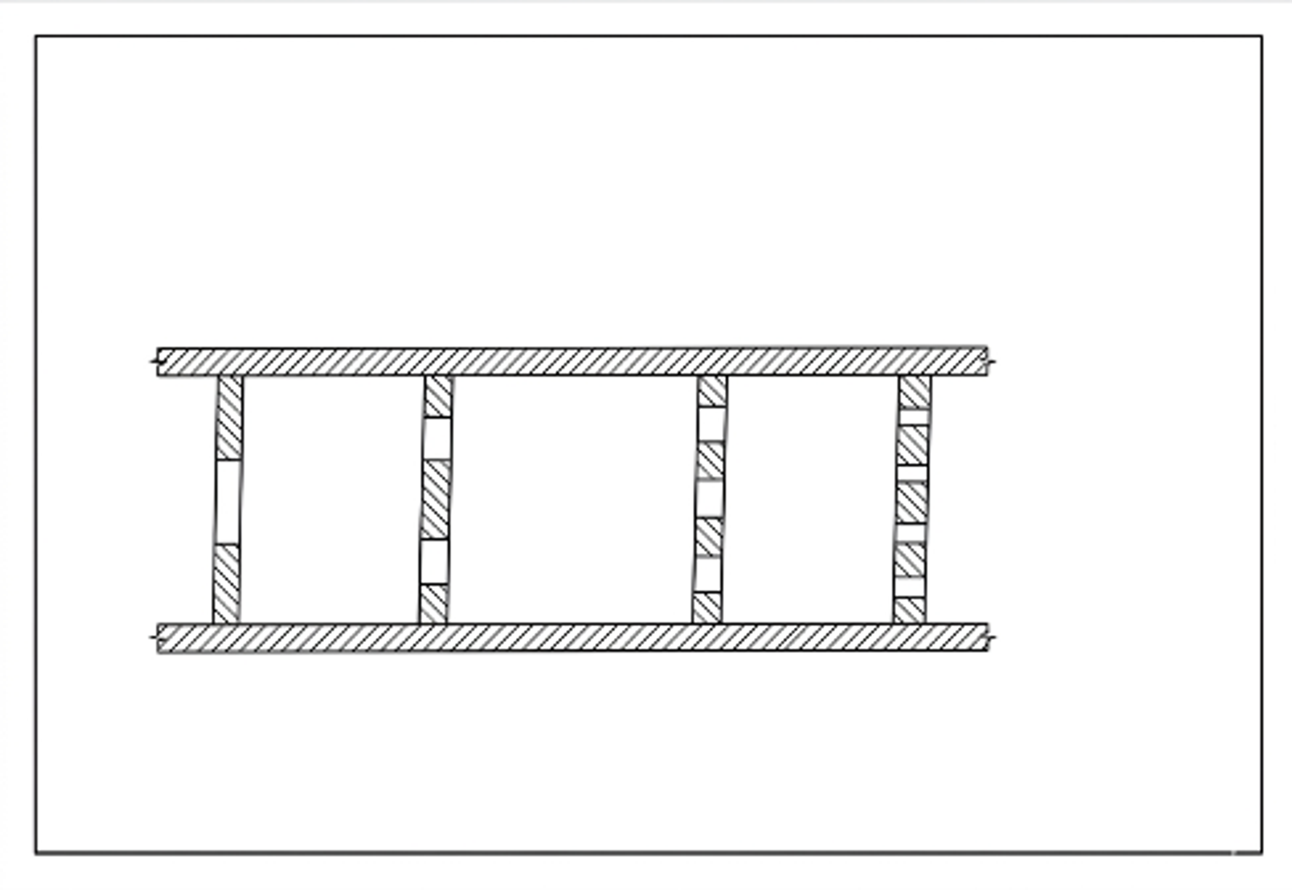
Rapid decompression overlaps with hydrodynamic cavitation but emphasizes a very rapid transition from a compressed suspension to a low pressure region. Pressure retained in liquid filled defects and pores can assist expansion, while constrictions generate high velocity jets and bubbles. Patent literature describes serial or parallel local restrictions, rotating cavitation zones, and pulsed or cavitating waterjets. Patent claims and examples should be treated as technical disclosures rather than as independent validation of commercial performance.
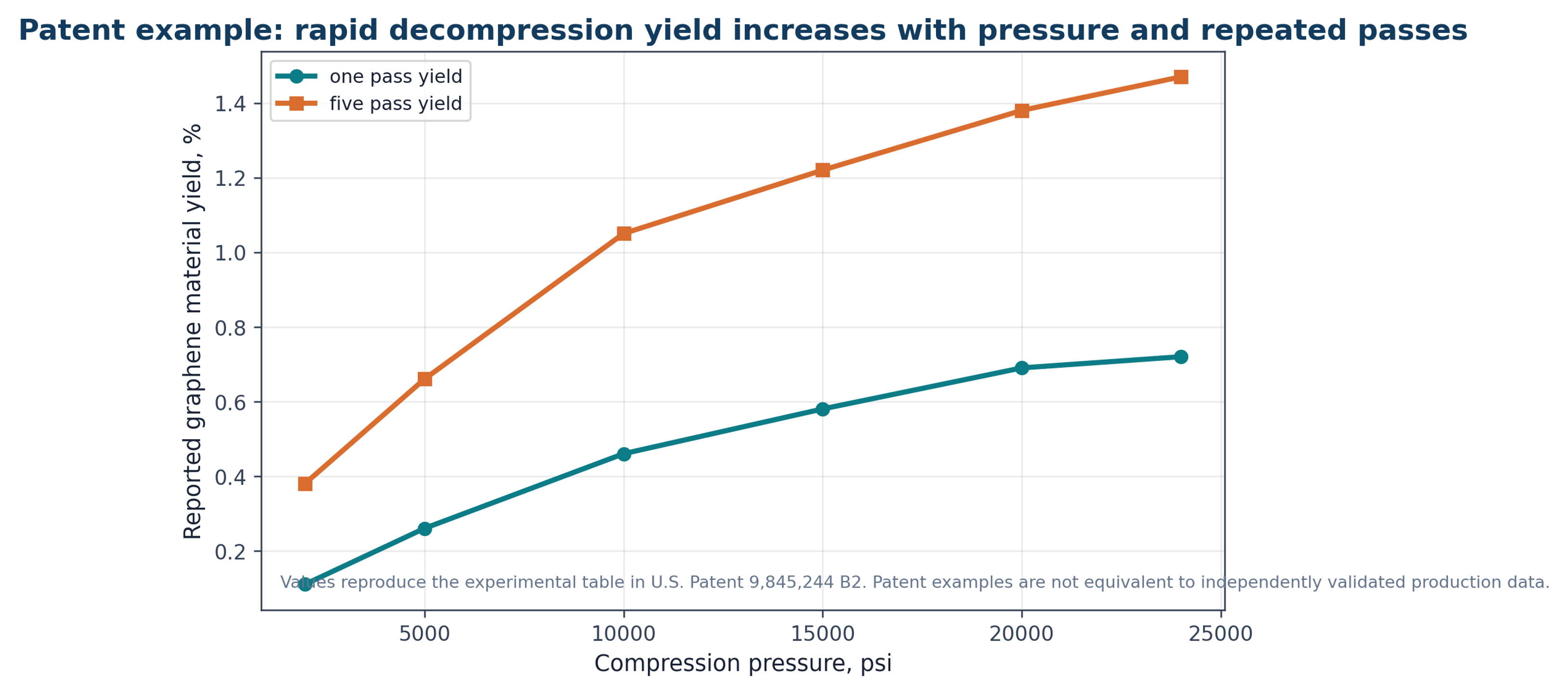
U.S. Patent 9,845,244 B2 describes compression followed by decompression to less than 20 percent of the compression pressure in less than 2 × 10⁻⁶ s to generate a cavitation event. An example table reports increasing one pass and five pass yields as compression pressure increases from 2,000 to 24,000 psi. The highest listed five pass value is 1.47 percent at 24,000 psi, while the specification discusses higher estimated yield after additional recirculation and optimization [23].
Figure 7.1. Reported yield values in the rapid decompression example [23]Source citation in original document: [23].
*[Figure 7.1](#figure-7-1). Reported yield values in the rapid decompression example [23].*
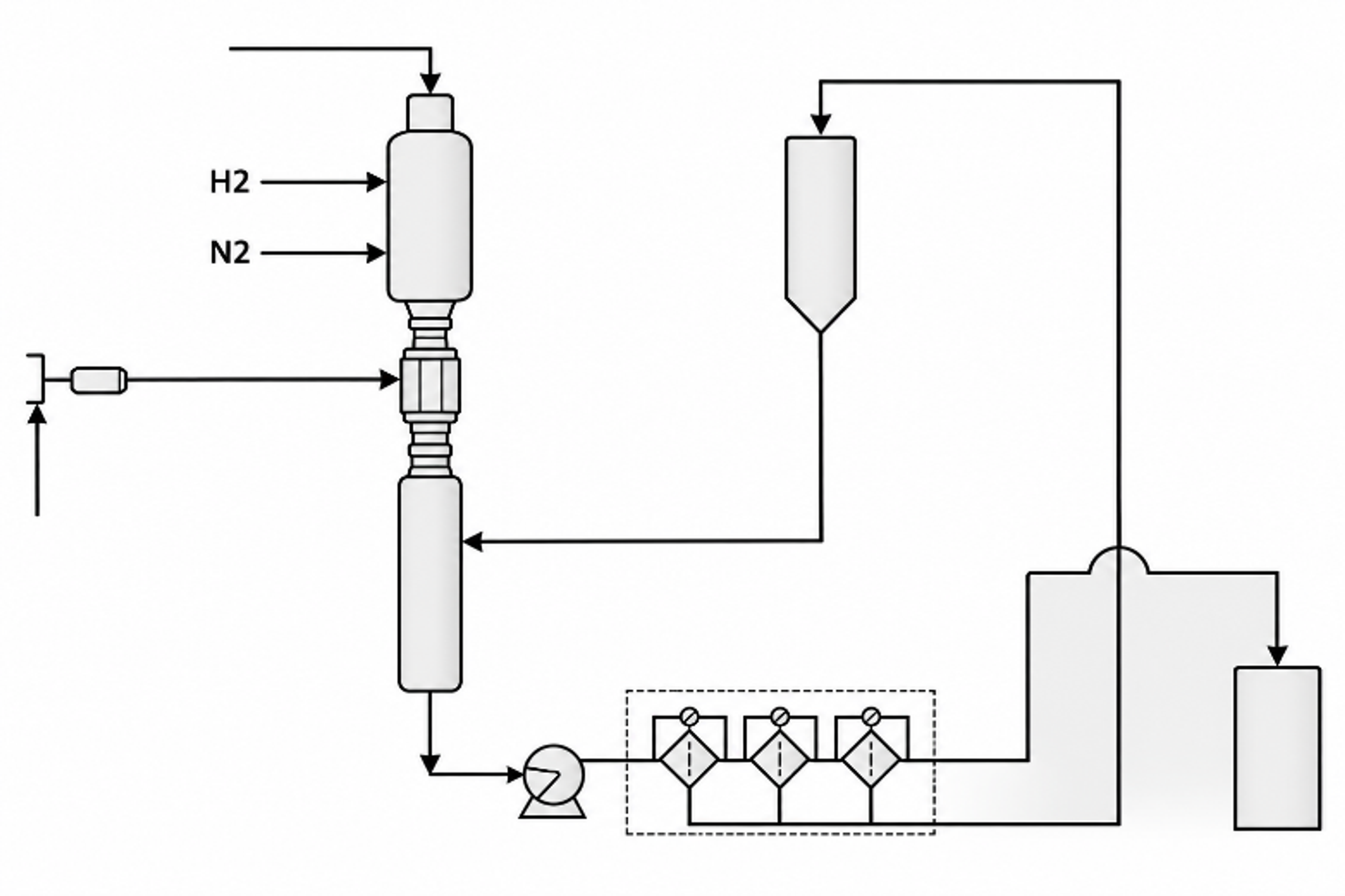
Figure 7.2. Patent flow diagram for mixing, compression, rapid decompression, and product separation [23]Source citation in original document: [23].
*[Figure 7.2](#figure-7-2). Patent flow diagram for mixing, compression, rapid decompression, and product separation [23].*
Figure 7.3. Schematic local restriction architecture for rapid decompression treatment [23]Source citation in original document: [23].
*[Figure 7.3](#figure-7-3). Schematic local restriction architecture for rapid decompression treatment [23].*
U.S. Patent 9,315,388 B2 describes production and possible concurrent functionalization in a controlled cavitating fluid. U.S. Patent Application 2018/0009667 describes high pressure or pulsed waterjet injection into an exfoliation chamber followed by filtration and collection [22,24]. The disclosed approaches overlap functionally but differ in reactor geometry, feed introduction, cavitation generation, and downstream handling.
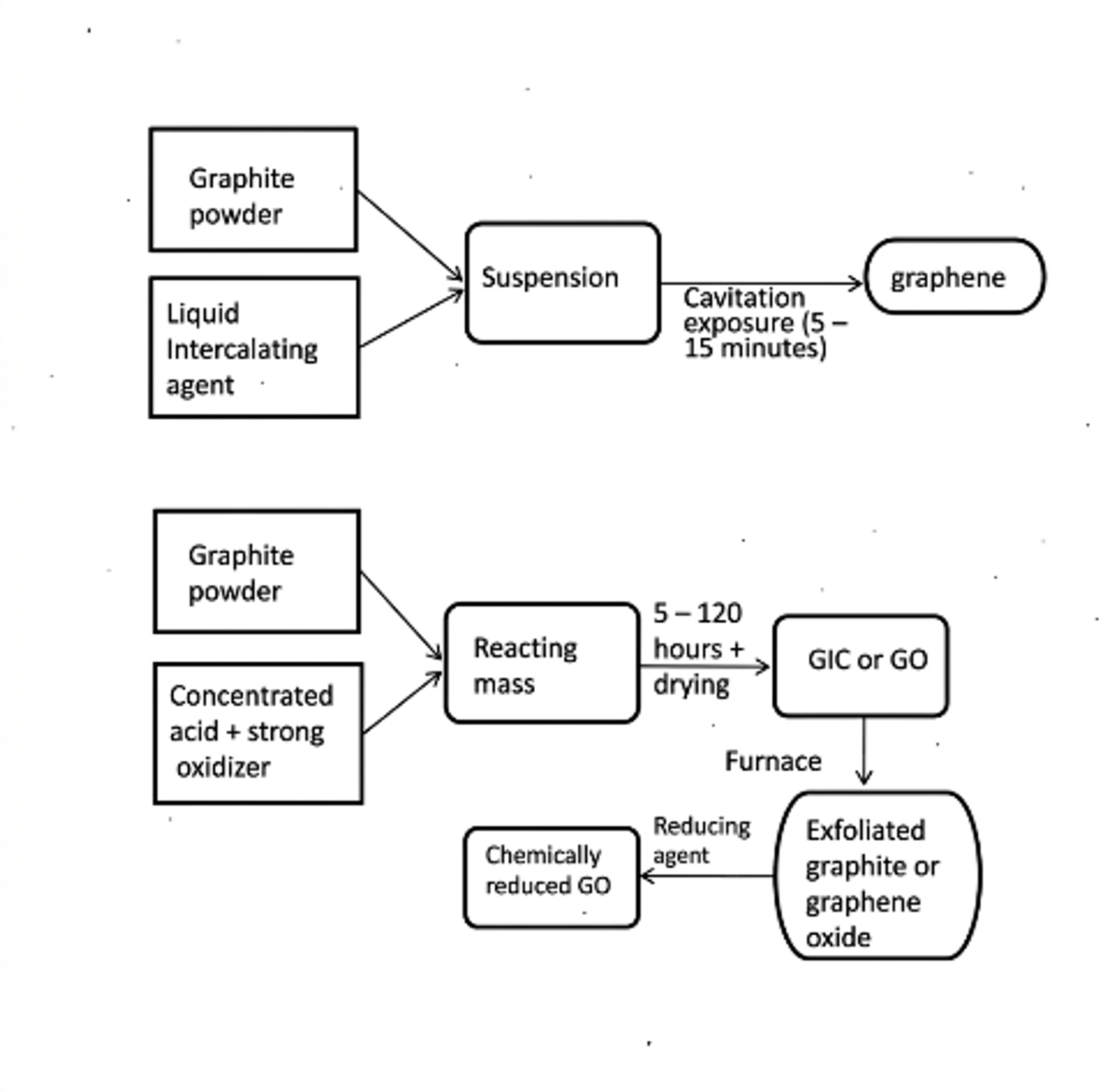
Figure 7.4. Patent comparison of a short cavitation exposure route with a longer oxidation and thermal route [22]Source citation in original document: [22].
*[Figure 7.4](#figure-7-4). Patent comparison of a short cavitation exposure route with a longer oxidation and thermal route [22].*
Figure 7.5. Pulsed or cavitating waterjet graphene preparation system with exfoliation chamber, separation, and collection [24]Source citation in original document: [24].
*[Figure 7.5](#figure-7-5). Pulsed or cavitating waterjet graphene preparation system with exfoliation chamber, separation, and collection [24].*
## 8 Microfluidization, Wet Jet Milling, Rotor Stator Processing, and Hybrid Routes
### 8.1 Microfluidization
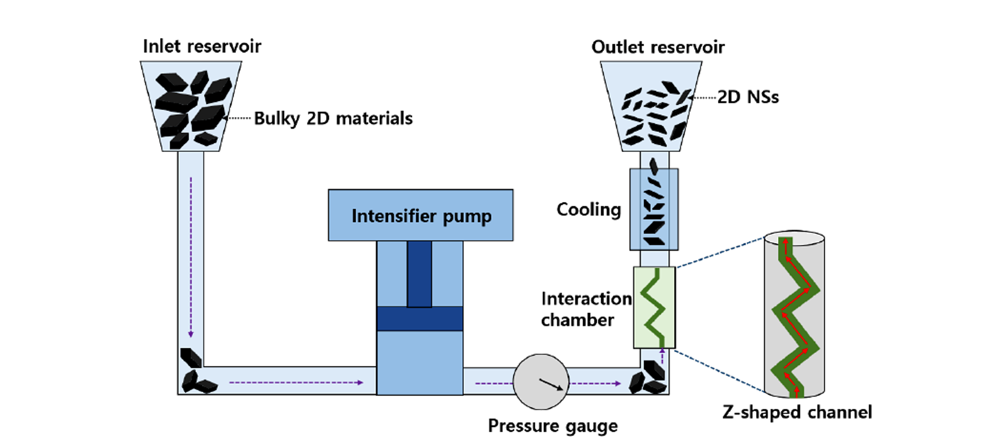
Microfluidization forces a suspension through a narrow interaction chamber at high pressure. A Z shaped or otherwise engineered channel can generate shear rates approaching 10⁸ s⁻¹ together with turbulence, collision, pressure release, and possible cavitation. Reported channel widths commonly range from approximately 87 to 400 micrometers [13,20,21]. Each pass is continuous and readily recirculated, but repeated cycling can narrow the thickness distribution while increasing edge density and eventually damaging basal planes.
Figure 8.1. General microfluidization system with feed reservoir, intensifier pump, interaction chamber, cooling section, and outlet reservoir [13]Source citation in original document: [13]. License stated in bibliography: CC BY 4.0.
*[Figure 8.1](#figure-8-1). General microfluidization system with feed reservoir, intensifier pump, interaction chamber, cooling section, and outlet reservoir [13].*
Karagiannidis and coauthors reported aqueous microfluidization at approximately 10⁸ s⁻¹ with graphite concentrations up to 100 g L⁻¹ and described 100 percent conversion to material with thickness below 70 nm without centrifugation yield loss. The resulting dispersions were formulated as conductive inks [21]. In that context, 100 percent yield does not mean 100 percent monolayer graphene. It refers to the defined processed nanosheet fraction and the absence of discarded coarse material. This distinction should be made explicit when commercial claims are compared.
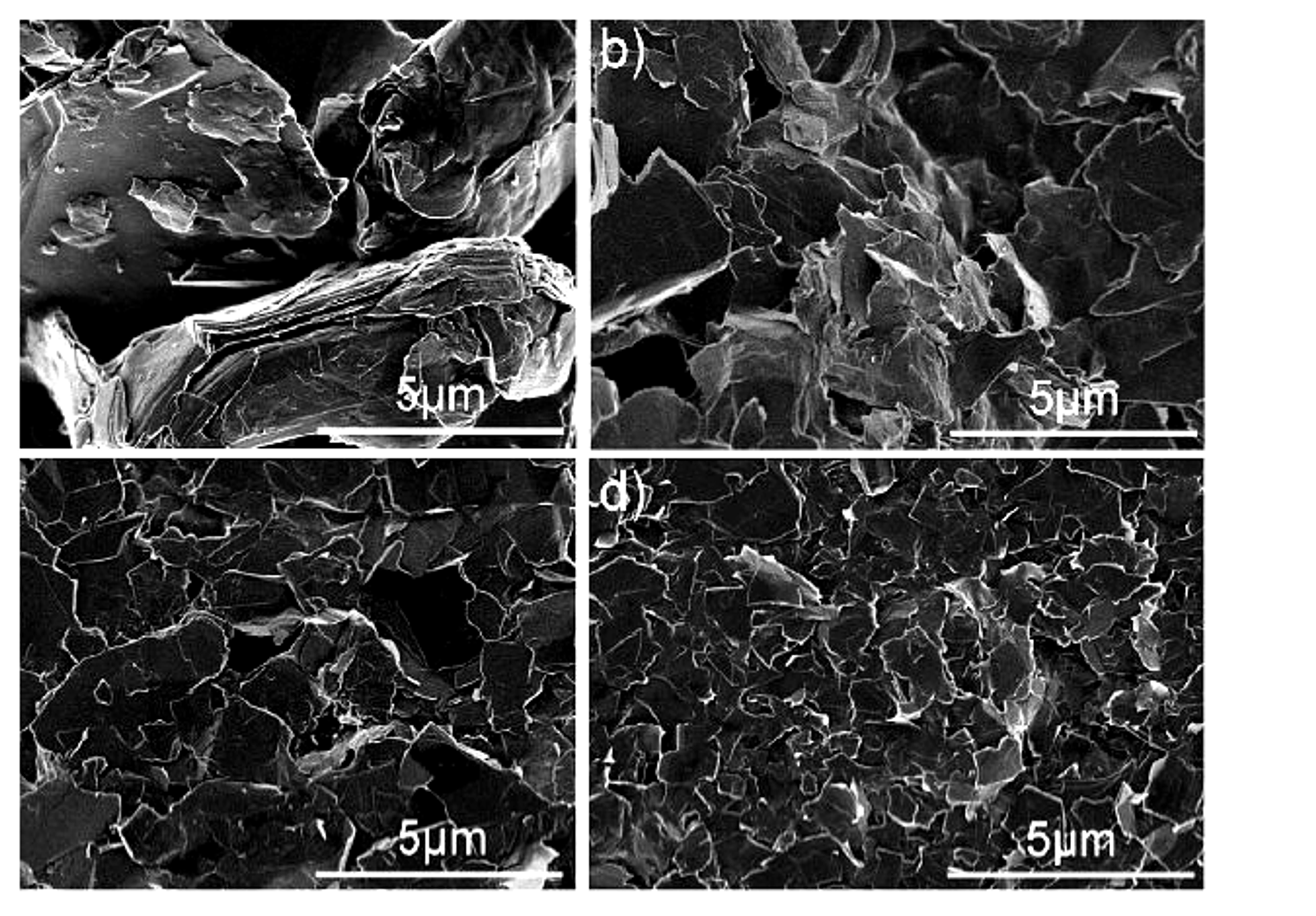
Figure 8.2. Images of graphite morphology after 0, 1, 5, and 100 passes through a Microfluidizer processor at 30,000 psi [20]Source citation in original document: [20].
*[Figure 8.2](#figure-8-2). Images of graphite morphology after 0, 1, 5, and 100 passes through a Microfluidizer processor at 30,000 psi [20].*
### 8.2 Wet Jet Milling
Wet jet milling drives a suspension through perforated disks, nozzles, or interacting jets at high pressure. The active stresses include shear at microchannel junctions, extensional flow, collision, and pressure release. The process has been applied to graphite, boron nitride, MoS₂, and WS₂ and is attractive because residence time per pass is short and throughput can be increased through pump capacity or parallelization [13]. Principal concerns include nozzle wear, blockage, pressure containment, high capital cost, flake cutting, and the need for effective cooling.
### 8.3 Rotor Stator High Shear Processing
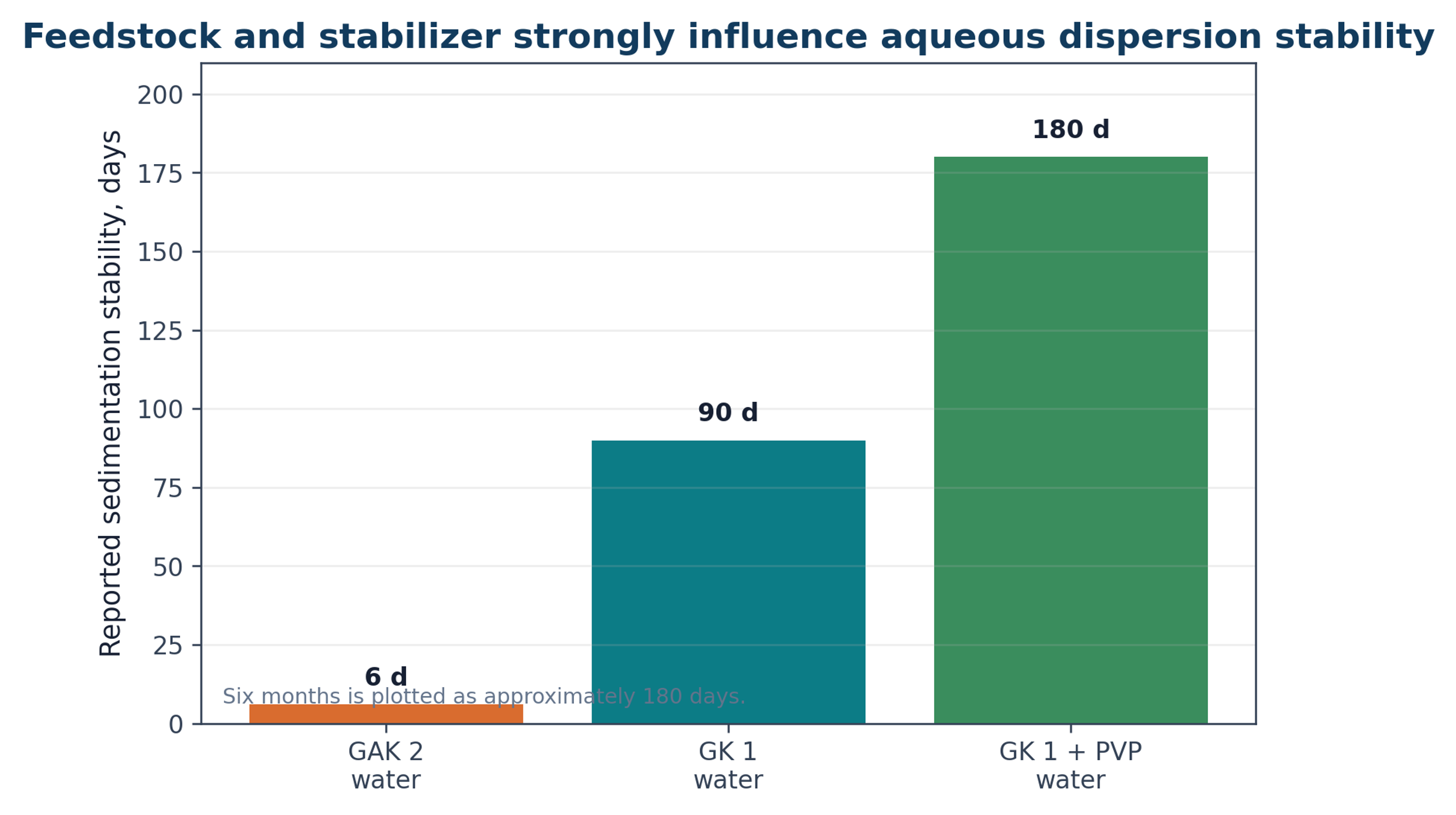
Rotor stator mixers generate high velocity gradients in a narrow gap, jets through stator openings, recirculation, and repeated particle collisions. Cavitation may occur locally, but shear and impact can dominate depending on geometry. A study using 40 volume percent isopropyl alcohol in water reported 0.27 mg mL⁻¹ graphene related nanosheets after 1 h, with most flakes below 1 micrometer lateral size and approximately 2 nm thickness [15]. A 2024 study using natural graphite in water at 4,000 to 11,000 rpm for 3 to 120 min showed that graphite grade and polyvinylpyrrolidone strongly influenced sedimentation stability, with reported stability ranging from 6 days to approximately 6 months [14].
Figure 8.3. Reported sedimentation stability for two natural graphite grades and a polyvinylpyrrolidone stabilized suspension [14]Source citation in original document: [14].
*[Figure 8.3](#figure-8-3). Reported sedimentation stability for two natural graphite grades and a polyvinylpyrrolidone stabilized suspension [14].*
### 8.4 Hybrid Processing
Hybrid routes use one operation to prepare the feed for another. Examples include mild expansion before cavitation, ultrasound before a hydrodynamic chip, rotor stator wetting before a high pressure pass, sequential nozzle sizes, dual frequency ultrasound, or functionalization after exfoliation. Hybridization can reduce the burden on the most expensive or damage intensive stage, but it adds equipment, control variables, cross contamination risk, and patent complexity.
*Table 8.1. Representative equipment for liquid exfoliation and cavitation processing.*
| **Equipment** | **Dominant mechanisms** | **Advantages** | **Main limitations** | **Best use** |
|----------------------------|---------------------------------------------------------------------------------|-------------------------------------------------------------|----------------------------------------------------------------------|-----------------------------------------------------------|
| Ultrasonic bath | Distributed low intensity acoustic cavitation. | Low cost and simple screening. | Poor power quantification and slow treatment. | Early solvent and stabilizer screening. |
| Probe sonicator | Localized high intensity acoustic cavitation and microstreaming. | Fast laboratory treatment and flexible amplitude control. | Nonuniform exposure, heating, tip erosion, metal contamination. | Mechanism studies and small batch optimization. |
| Ultrasonic flow cell | Acoustic cavitation in a defined flow residence. | Better reproducibility, cooling, and recycle control. | Field calibration and bubble shielding remain important. | Pilot development when acoustic treatment is required. |
| Venturi or orifice reactor | Pressure reduction, cavitation, turbulence, and recovery collapse. | Simple geometry and continuous operation. | Erosion, pressure loss, and broad residence time if poorly designed. | Moderate pressure hydrodynamic processing. |
| Jet cavitation device | High pressure nozzles, cavitation, shock waves, and turbulent jets. | Strong treatment and direct control by pressure and passes. | Pump cost, wear, heat generation, and flake fragmentation. | High intensity recirculating exfoliation. |
| Microfluidic chip | Defined constriction, cavitation visualization, and high local shear. | Excellent mechanistic control and low active volume. | Clogging and low absolute throughput without numbering up. | Mechanism, rapid screening, and controlled microreactors. |
| Microfluidizer | High shear, extensional flow, collision, pressure release, possible cavitation. | High solids potential and industrial equipment base. | High capital and wear; repeated passes can damage flakes. | Concentrated dispersions and ink manufacture. |
| Wet jet mill | High pressure jets, shear at junctions, collision, and pressure release. | Short pass time and broad 2D material applicability. | Nozzle wear, blockage, pressure containment, and cutting. | High throughput nanosheet production. |
| Rotor stator mixer | Gap shear, jets, turbulence, collision, and local cavitation. | Widely available, scalable, and easy to integrate. | Field is complex and product can be broad. | Premixing, deagglomeration, and moderate exfoliation. |
## 9 Extension to Other Two Dimensional Nanomaterials
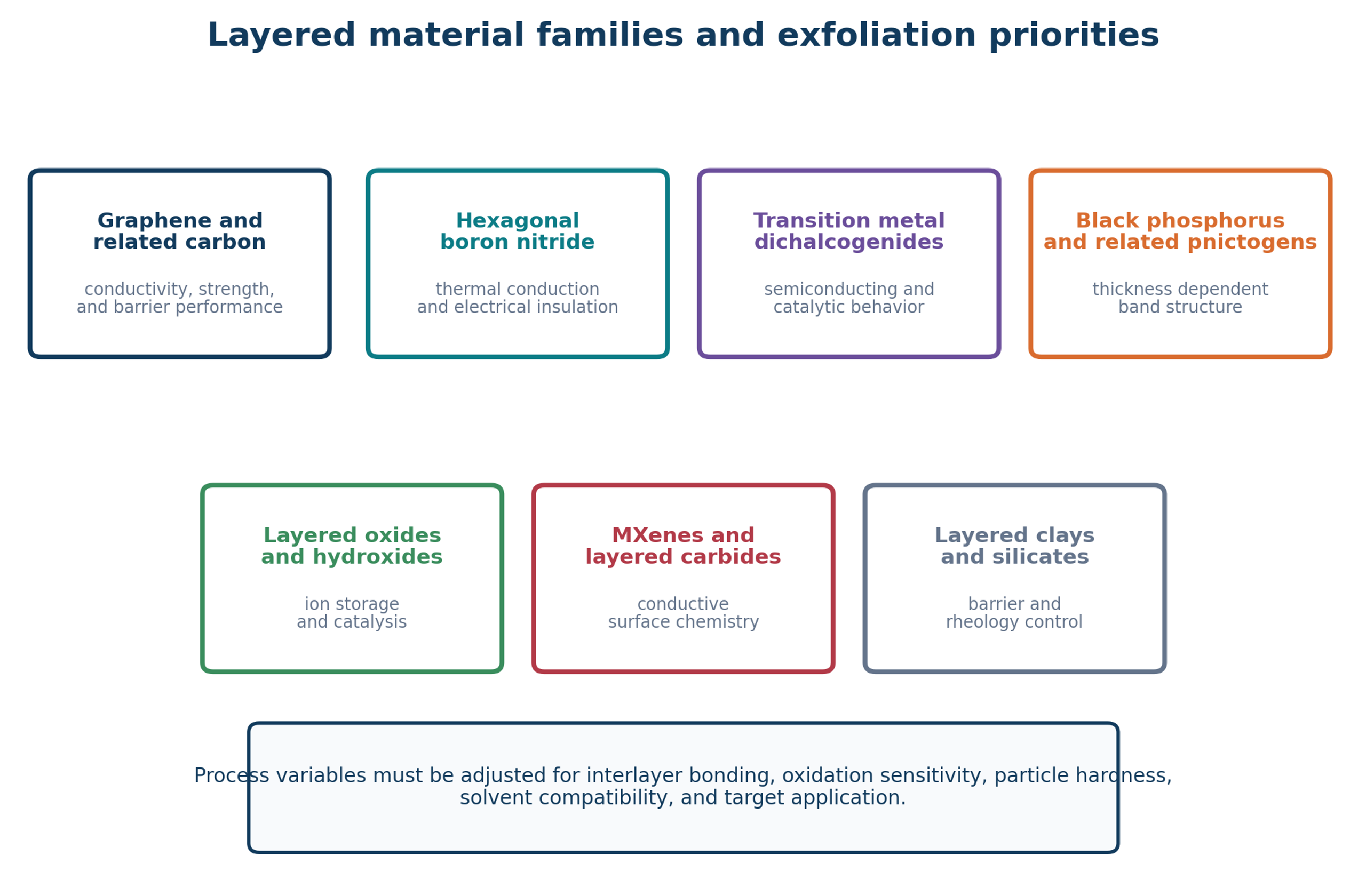
Figure 9.1. Major layered material families that can be processed by liquid exfoliation. Each family requires a different balance of stress, chemistry, oxygen control, and product stabilization [37]Source citation in original document: [37].
*[Figure 9.1](#figure-9-1). Major layered material families that can be processed by liquid exfoliation. Each family requires a different balance of stress, chemistry, oxygen control, and product stabilization [37].*
### 9.1 Hexagonal Boron Nitride
Hexagonal boron nitride is structurally analogous to graphite but is electrically insulating and thermally conductive. It is attractive for thermal management, electrically insulating composites, lubricants, coatings, and dielectric applications. Microfluidization has produced boron nitride nanosheets in minutes rather than the prolonged sonication often required by conventional methods [13]. Because boron nitride is harder and can be more abrasive than graphite, nozzle and pump wear, metal contamination, and classification require particular attention. The product specification should include electrical resistivity in addition to thickness and lateral size.
### 9.2 Transition Metal Dichalcogenides
MoS₂ and WS₂ combine layered structures with semiconducting, catalytic, and tribological behavior. Their layers are chemically more complex than graphene and may be sensitive to oxidation, phase change, edge chemistry, and stoichiometry. Ultrasonic MoS₂ studies show that increasing power does not always increase concentration because cavitation shielding and fragmentation change after an optimum [18]. Wet jet and microfluidic routes can rapidly produce few layer material [13]. Quality control should include Raman peak positions and widths, XPS oxidation state, elemental ratio, and application specific performance.
### 9.3 Black Phosphorus and Air Sensitive Materials
Black phosphorus and related materials require oxygen and moisture control because newly exfoliated surfaces can degrade rapidly. Cavitation increases interfacial area and can accelerate undesired chemistry. Processing may require deoxygenated solvent, inert gas blanketing, low temperature, rapid transfer, antioxidants, encapsulation, or immediate formulation. A reactor that performs well for graphite in water cannot be transferred directly to black phosphorus without a complete chemical risk assessment.
### 9.4 Layered Oxides, Hydroxides, MXenes, and Clays
Layered oxides and hydroxides are used in catalysis and energy storage, while MXenes provide conductive surfaces terminated by oxygen, hydroxyl, fluorine, or other groups. Clays and silicates are used for barrier performance, rheology modification, and reinforcement. These materials may swell, exchange ions, dissolve, change oxidation state, or react with water. Hydrodynamic stress can assist delamination, but solvent chemistry and pH can be more influential than cavitation intensity. Process development should separate chemical activation from mechanical separation so that the contribution of each can be measured.
*Table 9.1. Processing implications for selected two dimensional material families.*
| **Material family** | **Interlayer or surface issue** | **Promising liquid process** | **Additional quality controls** |
|--------------------------------------|-------------------------------------------------------------------------------|------------------------------------------------------------------------|----------------------------------------------------------------------------|
| Graphite and graphene related carbon | Restacking, edge damage, oxygen and metal contamination. | Cavitation, high shear, microfluidization, wet jet milling. | Raman, AFM, TEM, XPS, ash, conductivity, residual stabilizer. |
| Hexagonal boron nitride | Hard and abrasive; insulating product must remain low in metal contamination. | Microfluidization, wet jet, ultrasound, rotor stator. | Thickness, thermal conductivity, electrical resistivity, elemental purity. |
| MoS₂ and WS₂ | Stoichiometry, oxidation, phase changes, edge chemistry. | Ultrasound at controlled intensity, wet jet, microfluidic processing. | Raman, XPS, elemental ratio, catalytic or electronic performance. |
| Black phosphorus | Rapid oxidation and hydrolysis of thin sheets. | Inert, low temperature, closed acoustic or microfluidic process. | Oxygen content, degradation products, encapsulation quality. |
| Layered oxides and hydroxides | Swelling, ion exchange, dissolution, pH sensitivity. | Controlled shear or cavitation combined with chemical conditioning. | Phase identity, oxidation state, composition, ion release. |
| MXenes | Surface termination, oxidation, and colloidal stability. | Gentle deagglomeration and classification after chemical delamination. | Surface terminations, oxidation, conductivity, flake size. |
| Clays and silicates | Swelling and ion exchange dominate separation. | Hydration, chemical conditioning, rotor stator or moderate cavitation. | Aspect ratio, mineral phases, exchange capacity, rheology. |
## 10 Feed Preparation, Process Chemistry, and Contamination Control
### 10.1 Graphite Feedstock Qualification
Natural graphite grade, crystallinity, particle size, morphology, ash, moisture, metal content, and prior processing can substantially alter exfoliation behavior. Large crystalline flakes can provide large nanosheets but may clog small channels. Fine graphite disperses readily but may already contain defects and can produce smaller platelets. Expanded graphite lowers interlayer resistance but adds pretreatment and may introduce residual intercalants. Synthetic graphite offers greater consistency but may differ in crystallite size and cost. A feed specification should include, at minimum, particle size distribution, ash, moisture, elemental impurities, XRD crystallinity, and a reference exfoliation test.
(10.1)
d95 is the 95th percentile feed particle size, Dh is the minimum hydraulic diameter, and κ is a conservative blockage ratio selected from geometry and particle shape. For rigid irregular flakes, κ may need to be well below 0.1.
### 10.2 Premixing and Deagglomeration
Dry powder should not be introduced directly into a high pressure microchannel unless the feeding and wetting system is designed for that duty. Premixing should eliminate floating agglomerates, wet particle surfaces, dissolve the stabilizer, and produce reproducible viscosity. Low speed agitation, rotor stator mixing, recirculation through a coarse bypass, or vacuum wetting can be used. The premix should be sampled before exfoliation so that subsequent changes are not confused with variation in feed dispersion.
### 10.3 Contamination Sources
Metal contamination can originate from sonotrodes, valves, nozzles, pumps, bearings, rotor stator surfaces, and collection vessels. Polymer fragments can originate from seals, hoses, and filters, while silica or ceramic particles can originate from interaction chambers. Contamination should be monitored by ICP MS, ash analysis, SEM with elemental analysis, and blank runs. Equipment material selection must account for abrasion as well as corrosion. A process that produces excellent Raman spectra but introduces unacceptable nickel, iron, titanium, or ceramic contamination is unsuitable for electronic, biomedical, or catalytic products.
## 11 Post Processing, Classification, Concentration, and Formulation
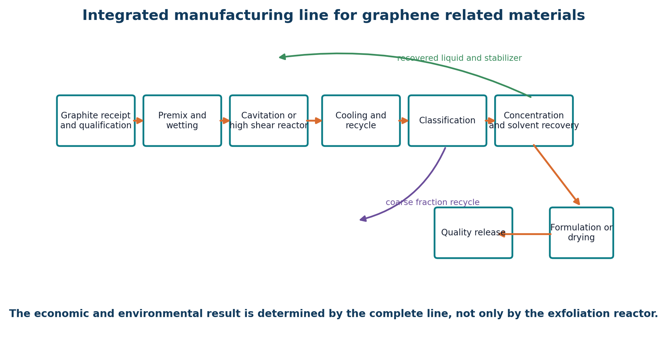
Exfoliation is only the first unit operation. Reactor output generally contains unexfoliated graphite, thick nanosheets, target material, fines, dissolved stabilizer, wear particles, and gas bubbles. Classification determines the actual product distribution and often dominates usable yield. Centrifugation, sedimentation, membrane filtration, cross flow filtration, hydrocyclones, decantation, and selective flocculation can be used individually or in sequence.
Figure 11.1. Integrated manufacturing line from feed qualification to product release. Recycle and solvent recovery are part of the process definition [37]Source citation in original document: [37].
*[Figure 11.1](#figure-11-1). Integrated manufacturing line from feed qualification to product release. Recycle and solvent recovery are part of the process definition [37].*
### 11.1 Centrifugal Classification
Centrifugal classification is widely employed for separating and fractionating suspended particulate matter, such as exfoliated nanosheets, based on sedimentation behavior. The relative centrifugal force (, expressed in units of ) is a function of the rotational radius (in centimetres) and the rotational speed (in revolutions per minute):
(11.1)
RCF is relative centrifugal force in units of g, r is rotational radius in centimetres, and n is rotational speed in revolutions per minute. Reporting rpm without radius is insufficient.
The Stokes settling velocity () for an equivalent spherical particle of diameter is given by:
(11.2)
where is the density difference between the dispersed phase and the medium, and is the dynamic viscosity of the liquid. Because anisotropic structures such as platelets and nanosheets deviate significantly from ideal spheres, this equation serves only as a preliminary screening approximation.
A centrifugal cascade can remove the largest particles at low acceleration and then collect a selected nanosheet fraction at higher acceleration. Every centrifugation step changes both product quality and yield. The complete protocol should state rotor radius, relative centrifugal force, time, temperature, collected fraction, and concentration method. Two laboratories can report different yields from identical reactor output solely because one uses a more severe separation protocol.
### 11.2 Membranes and Cross Flow Filtration
Membranes can concentrate nanosheets and recover solvent, but cake formation and irreversible fouling are common. Cross flow operation reduces cake growth and can support continuous processing. Membrane materials must tolerate the solvent and stabilizer and should not shed particles. A staged design can use a coarse protective filter, a product retention membrane, and a solvent polishing step. Both permeate and retentate should be included in the solids balance.
### 11.3 Drying and Redispersion
Drying can cause irreversible restacking. Spray drying, freeze drying, vacuum drying, drum drying, and direct masterbatch production create different agglomerate structures. When the final application is a liquid formulation or polymer composite, avoiding dry powder may be preferable. Concentrated paste or masterbatch formats reduce dust exposure and can preserve dispersion. Redispersion energy and final application performance should be measured after any drying route.
### 11.4 Formulation and Application Conversion
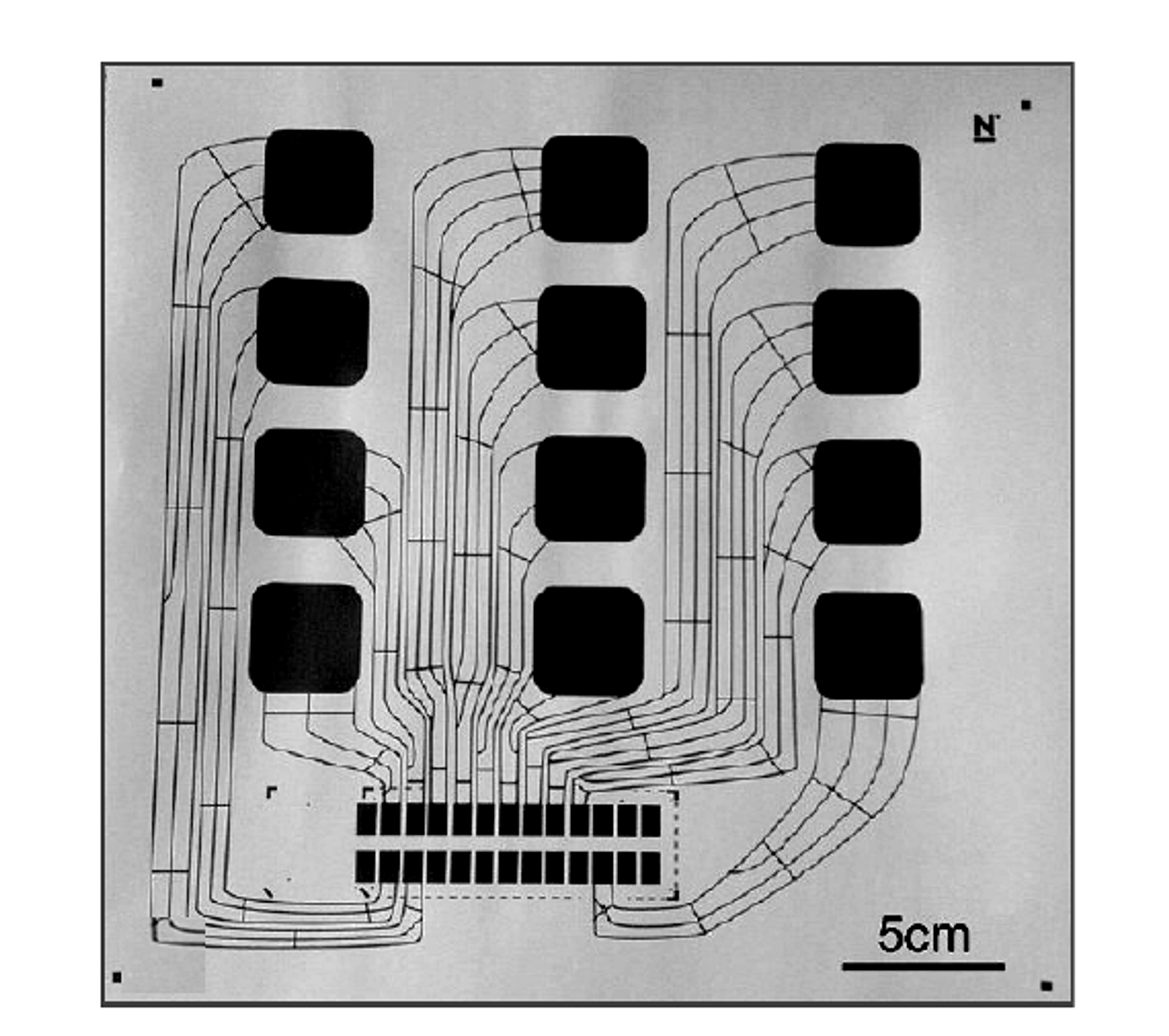
Printed electronics require controlled viscosity, surface tension, particle size relative to the nozzle or screen, conductivity after drying, adhesion, and flexibility. A Microfluidizer application note reported printed features near 100 micrometers and conductivity up to 2 × 10⁴ S m⁻¹ in a case study, while structural distortion was reported above approximately 70 cycles [20]. These values are useful process indicators but remain supplier reported and formulation specific.
Figure 11.2. Printed capacitive circuit prepared from microfluidized graphene ink [20]Source citation in original document: [20].
*[Figure 11.2](#figure-11-2). Printed capacitive circuit prepared from microfluidized graphene ink [20].*
*Table 11.1. Downstream operations and their influence on product quality.*
| **Operation** | **Primary purpose** | **Key control variables** | **Main risk** |
|----------------------------------|----------------------------------------------------------|------------------------------------------------------------------|------------------------------------------------------------------|
| Low acceleration centrifugation | Remove unexfoliated graphite and large fragments. | RCF, time, temperature, fill volume, collected fraction. | Loss of large but thin flakes and inconsistent decanting. |
| High acceleration centrifugation | Collect or sort thin nanosheets. | RCF distribution, rotor geometry, time, density and viscosity. | Low throughput and difficult scale up. |
| Membrane filtration | Concentrate product and recover liquid. | Pore size, transmembrane pressure, cross flow velocity, fouling. | Cake formation, membrane shedding, irreversible loss. |
| Sedimentation or decantation | Low cost removal of unstable coarse material. | Time, temperature, container geometry, stabilizer. | Slow operation and sensitivity to vibration and convection. |
| Drying | Produce powder for storage or compounding. | Droplet size, temperature, pressure, residual solvent. | Restacking, oxidation, dust, and poor redispersion. |
| Paste or masterbatch production | Avoid dry powder and deliver application ready material. | Carrier compatibility, solids loading, rheology, mixing history. | Product becomes carrier specific and may hide nanosheet quality. |
| Solvent recovery | Reduce cost and environmental burden. | Recovery fraction, purity, energy, stabilizer carryover. | Accumulation of impurities in recycle. |
## 12 Characterization and Quality Assurance
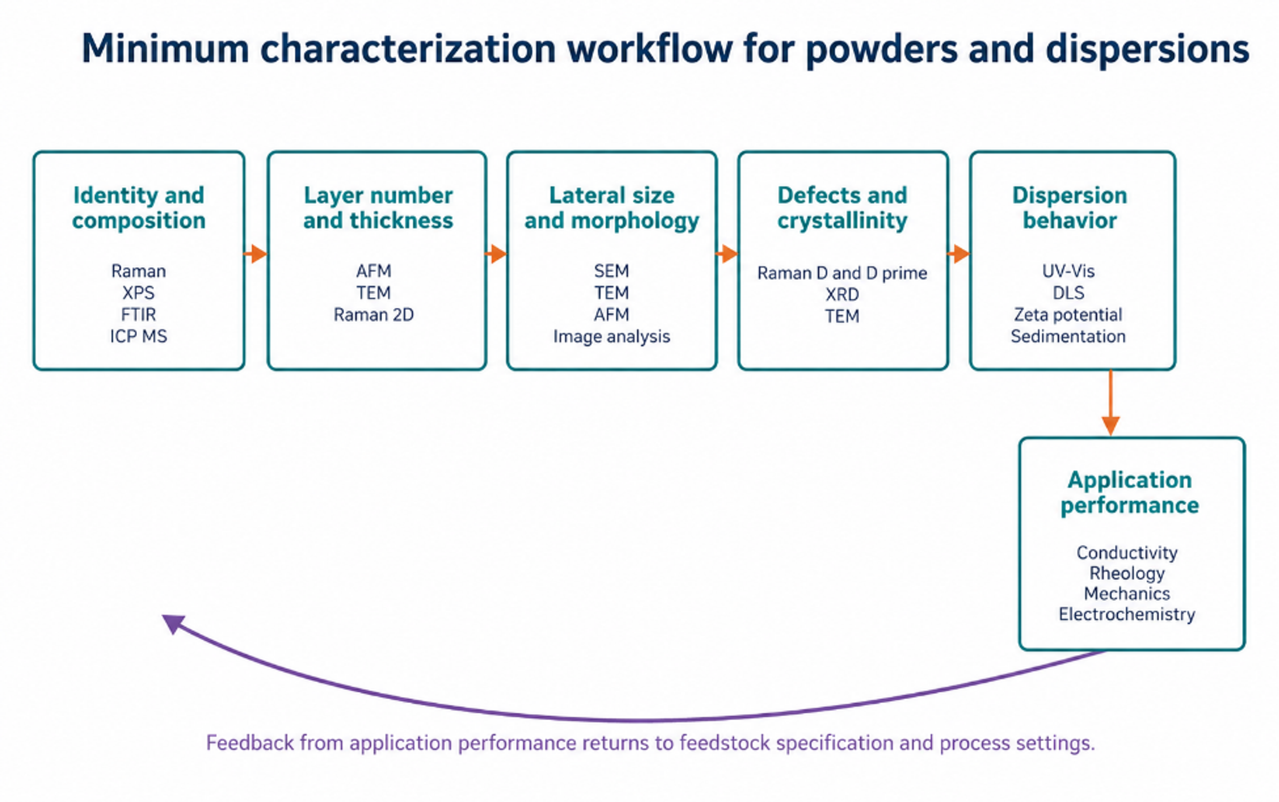
No single analytical method can establish that an industrial batch satisfies a graphene specification. Raman spectroscopy is rapid but samples a limited area and can confound edge related D band intensity with basal plane disorder. AFM measures thickness directly but has low throughput and is sensitive to substrate artifacts. TEM provides lattice and layer information but samples a very small mass. SEM covers a larger field but does not directly resolve monolayer thickness. XPS measures surface chemistry, ICP MS identifies trace metals, and UV Vis can estimate dispersed concentration only when the extinction coefficient and scattering conditions are appropriate. A defensible release specification therefore combines complementary methods [2,4,5,7-13].
Figure 12.1. Minimum characterization workflow connecting identity, structure, defects, dispersion behavior, and application performance [37]Source citation in original document: [37].
*[Figure 12.1](#figure-12-1). Minimum characterization workflow connecting identity, structure, defects, dispersion behavior, and application performance [37].*
### 12.1 Raman Spectroscopy
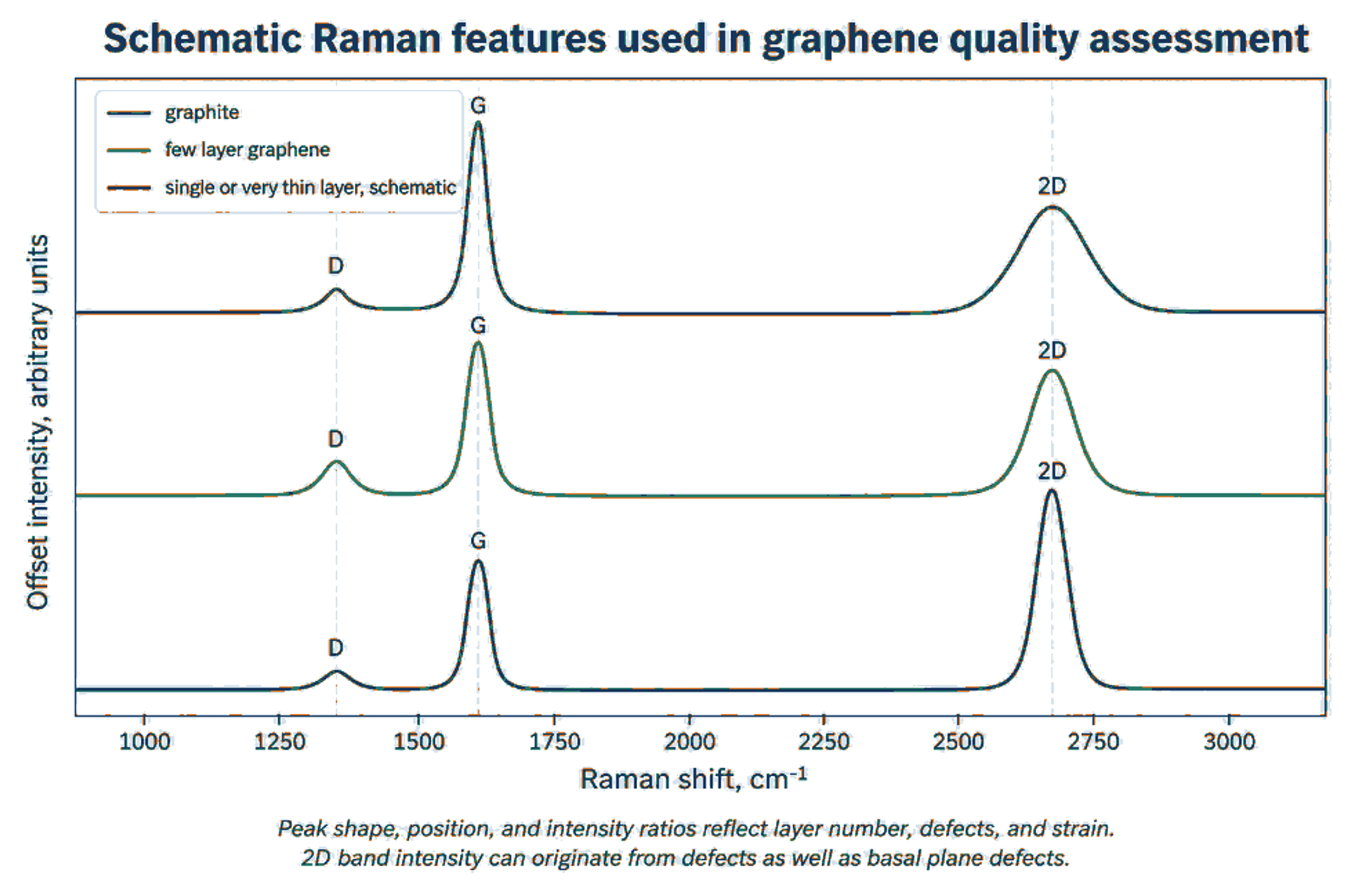
The principal Raman features are the D band near 1350 cm⁻¹, the G band near 1580 cm⁻¹, the D prime band near 1620 cm⁻¹, and the 2D band near 2700 cm⁻¹. Exact positions depend on excitation wavelength, strain, doping, temperature, and material condition. The D band is activated by disorder and edges. The 2D band shape and intensity provide layer information, but the relationship is not universal for all flake sizes and substrates. Raman mapping across many locations is more representative than a single selected spectrum [2].
Figure 12.2. Schematic Raman response for graphite, few layer graphene, and very thin graphene. The curves are educational and do not represent one measured batch [2]Source citation in original document: [2].
*[Figure 12.2](#figure-12-2). Schematic Raman response for graphite, few layer graphene, and very thin graphene. The curves are educational and do not represent one measured batch [2].*
Equation (12.1) generalized Tuinstra-Koenig relation used in Raman spectroscopy to determine the in-plane crystallite size () of nanographite, graphene, and other carbon-based materials:
(12.1)
La is an empirical in plane crystallite or defect spacing estimate in nanometers for a specified defect regime, λL is laser wavelength in nanometers, and ID/IG is the D to G intensity ratio. The equation must not be applied outside its calibration regime.
An increase in ID/IG during cavitation does not by itself prove increasing basal plane damage. If lateral size becomes smaller than the laser spot, a larger fraction of edges contributes to the D band. G band broadening, D prime behavior, peak position, mapping statistics, AFM size, and TEM observations should be considered together. The jet cavitation study attributed much of its D band increase to edge generation because strong G band broadening was not observed [9].
Figure 12.3. Raman spectra after 20, 40, 60, and 80 hydrodynamic cavitation cycles, showing increasing D band response and a 2D band shift after 80 cycles [11]Source citation in original document: [11]. License stated in bibliography: CC BY 3.0.
*[Figure 12.3](#figure-12-3). Raman spectra after 20, 40, 60, and 80 hydrodynamic cavitation cycles, showing increasing D band response and a 2D band shift after 80 cycles [11].*
### 12.2 Microscopy and Thickness Statistics
AFM thickness measured for a monolayer on a substrate is often greater than the nominal carbon layer spacing because of adsorbed water, residual stabilizer, trapped solvent, substrate interactions, and instrument calibration. A layer classification rule should therefore be validated with reference material and supported by Raman or TEM. Reported statistics should include the number of flakes measured, sampling locations, threshold definitions, and both number weighted and mass weighted distributions. A small number of selected monolayer images cannot represent batch yield.
(12.2)
N is an approximate layer count, is AFM measured thickness after accounting for substrate and adsorbate offset, and h0 is the calibrated apparent thickness per layer. The calibration should be established for the specific substrate and sample preparation. The equivalent aspect ratio, , is defined by the projected flake area, , and flake thickness, :
(12.3)
Using an area equivalent diameter avoids selecting an arbitrary length for irregular flakes.
### 12.3 Concentration and Dispersion Stability
Equation (12.4) is the Beer-Lambert relation used to connect optical attenuation with the concentration of a dispersed material. In fluid analysis and nanoparticle suspensions, the relation is widely used for spectrophotometric concentration measurements when the extinction coefficient and scattering conditions are validated for the specific formulation.
(12.4)
is absorbance at wavelength λ, is the extinction coefficient for the specific material and dispersion, C is concentration, and l is optical path length.
Equation (12.5) defines the normalized conconcentration ratio:
(12.5)
S(t) is a normalized dispersion stability index based on dispersed concentration at time t relative to the initial concentration . The sampling height and method must be fixed.
Extinction coefficients vary with flake size, thickness, stabilizer, scattering, and instrument geometry. A coefficient obtained from another formulation should not be applied without validation by gravimetry or an independent mass balance. Stability should be measured at the intended storage concentration and temperature because dilution can change adsorption equilibrium and produce a misleading result.
### 12.4 Chemical Purity and Trace Contamination
ISO/TS 23359:2025 identifies XPS, TGA, ICP MS, and FTIR among the methods used for chemical characterization of powders and liquid dispersions [5]. XPS provides surface elemental composition and oxygen bonding information. TGA quantifies volatile material, stabilizer content, and oxidation behavior. ICP MS detects trace metals from feedstock and equipment, while FTIR identifies major functional groups and residual organics. These measurements should be linked to application limits rather than reported only as descriptive spectra.
*Table 12.1. Recommended quality control metrics for cavitation exfoliation products.*
| **Attribute** | **Primary methods** | **Report as** | **Why it matters** |
|---------------------------|-----------------------------------------------------------------------------------|-----------------------------------------------------------------------------|----------------------------------------------------------------------------------|
| Layer number or thickness | AFM, TEM, Raman, XRD for bulk context. | Distribution, median, percent below defined thresholds. | Controls electronic, optical, barrier, and surface behavior. |
| Lateral size | SEM, TEM, AFM, validated image analysis, DLS as supporting method. | Number and area weighted distributions. | Controls aspect ratio, percolation, printability, reinforcement, and filtration. |
| Defects and crystallinity | Raman mapping, TEM, XRD. | ID/IG, D prime behavior, peak widths, map statistics, lattice observations. | Distinguishes useful edges from unacceptable basal plane damage. |
| Surface chemistry | XPS, FTIR, TGA. | Atomic composition, O/C, functional groups, organic residue. | Controls compatibility, conductivity, stability, and reactivity. |
| Trace metals and ash | ICP MS, ICP OES, ash, SEM EDS. | Mass fraction by element and total ash. | Critical for electronics, catalysis, biomedical use, and color. |
| Specific surface area | Gas adsorption with stated model and degassing. | m² g⁻¹ with uncertainty. | Relates to accessible surface and aggregation. |
| Dispersion stability | UV Vis, sedimentation, zeta potential, rheology. | Concentration retention with time and redispersion energy. | Determines storage, pumping, coating, and formulation life. |
| Application performance | Electrical, thermal, mechanical, rheological, electrochemical, or catalytic test. | Performance against control at fixed loading and processing. | Confirms that material metrics translate to value. |
## 13 Mass Balance, Yield Definitions, and Energy Efficiency
Yield is one of the least consistently defined quantities in the exfoliation literature. A process may report the mass remaining in a supernatant, the mass below ten layers, the mass below a specified thickness threshold, the mass recovered after drying, or the mass converted from starting graphite. These quantities answer different questions. Every report should state the numerator, denominator, separation protocol, and whether residual surfactant or stabilizer has been subtracted.
(13.1)
is usable product yield, is dry product mass meeting the complete specification after subtracting nonproduct residue, and m0 is dry starting layered solid.
(13.2)
Rp is usable production rate, and t is total elapsed process time, including recycle and required separation when comparing complete processes.
(13.3)
is mass of in specification product per unit system energy. includes reactor, pump, cooling, mixing, classification, and recovery energy within the stated system boundary.
A complete solids balance tracks the distribution across the product mass , coarse recycle or reject , fines , and unaccounted losses :
(13.4)
Each stream should be measured or bounded.
Energy per liter can make a dilute process appear efficient even when little usable product is recovered. Energy per kilogram of in specification product reveals the combined effect of solids loading and yield. Conversely, an energy per kilogram metric can favor a concentrated but low quality product if the specification is weak. Energy metrics must therefore be reported together with thickness, lateral size, defect level, purity, and application performance.
*Table 13.1. Minimum reporting basis for yield and energy comparison.*
| **Category** | **Required information** | **Preferred metric** |
|--------------------|------------------------------------------------------------------------------------------------------|-------------------------------------------------------|
| Feed | Dry solids mass, concentration, particle size, grade, moisture, ash, stabilizer. | Mass and composition at reactor inlet. |
| Reactor | Geometry, pressure or acoustic conditions, flow, temperature, active volume, residence time, passes. | Energy density and residence time distribution. |
| Separation | All centrifuge, membrane, settling, and filtration settings. | Recovery of each fraction and solids balance. |
| Product definition | Thickness, lateral size, defect, chemistry, and purity limits. | Mass meeting the complete specification. |
| Energy boundary | Pump, ultrasound, cooling, mixing, separation, drying, solvent recovery. | kWh kg⁻¹ usable product and kWh L⁻¹ processed liquid. |
| Throughput | Continuous or batch time, cleaning, sampling, and downtime. | kg h⁻¹ usable product at stated availability. |
| Uncertainty | Sampling, concentration, moisture, residue, and measurement error. | Confidence interval for yield and energy. |
## 14 Scale Up, Process Control, and Equipment Reliability
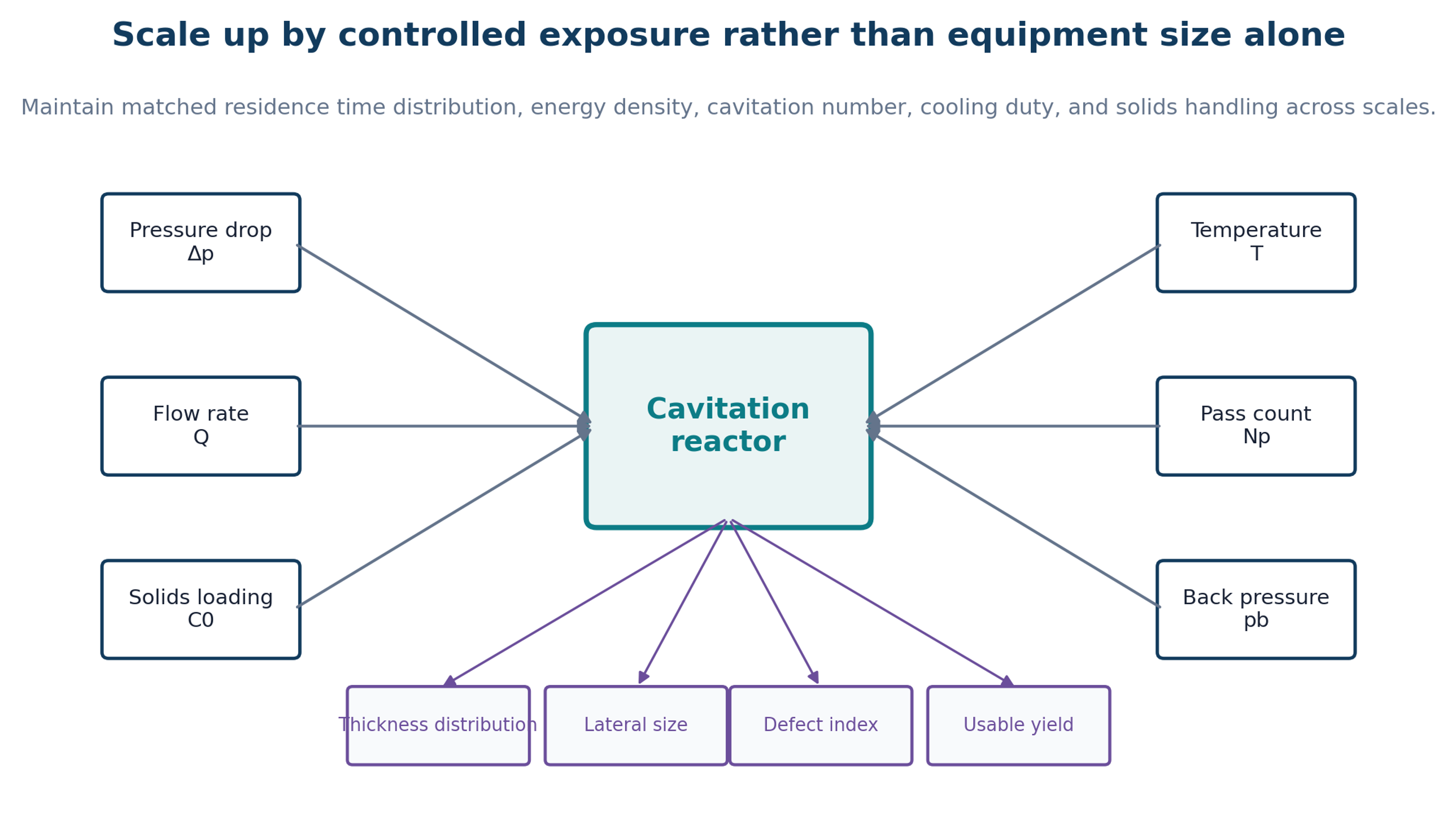
Scale up should preserve the distribution of effective exposure rather than geometric similarity alone. A larger reactor can have the same average pressure drop but a different cavity cloud, pressure recovery zone, particle trajectory, and residence time distribution. Likewise, a larger ultrasonic vessel can have the same power per liter but substantially poorer field uniformity. Scale up should therefore combine dimensionless groups, measured local signals, and product response.
Figure 14.1. Scale up variables and product responses. Pressure drop, flow, solids loading, temperature, pass count, and back pressure must be controlled as a coupled system [37]Source citation in original document: [37].
*[Figure 14.1](#figure-14-1). Scale up variables and product responses. Pressure drop, flow, solids loading, temperature, pass count, and back pressure must be controlled as a coupled system [37].*
Eu is an Euler pressure coefficient :
(14.1)
Eu is a Euler type pressure coefficient that helps compare pressure driven geometries. It should be considered together with Reynolds number, cavitation number, and residence time.
(14.2)
is nominal residence time in the active region, Vactive is active flow volume, and Q is flow rate. A residence time distribution is preferable to one nominal value.
(14.3)
is cumulative nominal exposure for Np passes. Damage can depend on the interval between passes and thermal history, so equal cumulative time does not always produce equal material.
### 14.1 Inline Sensing
Pressure transducers upstream, within the throat or nozzle, and downstream can identify flow regime and wear related drift. Flow meters verify exposure, temperature sensors quantify cooling duty, and hydrophones or structure borne acoustic sensors can track cavitation emission. Optical absorbance or turbidity can follow dispersed solids, while inline particle imaging or focused beam reflectance can track disappearance of large particles. Conductivity, density, viscosity, and dissolved gas measurements can reveal formulation changes. A control model should use these signals to maintain a product response rather than a fixed valve position.
### 14.2 Wear, Erosion, and Maintenance
Cavitation collapse and abrasive graphite attack nozzles, valve seats, interaction chambers, and pump components. Wear changes geometry and therefore changes pressure drop and product quality before a catastrophic failure becomes visible. Maintenance should be condition based. Pressure flow curves, acoustic signatures, metal contamination, and dimensional inspection can provide early warning. Replaceable inserts and modular parallel channels can reduce downtime.
(14.4)
ER is a simple erosion rate based on component mass loss Δm, exposed area A, and operating time t. Dimensional loss at the critical throat may be a more sensitive measure than total mass loss.
### 14.3 Cleaning and Product Changeover
Graphene strongly colors process surfaces and can remain in dead legs, seals, filters, and heat exchangers. Cleaning validation should define acceptable carryover according to the next product. A clean in place sequence may include draining, a compatible solvent flush, dispersant or alkaline washing where materials permit, a high velocity rinse, a filtered water or solvent rinse, and verification by absorbance or total carbon. Cleaning liquid must be included in the mass and environmental balance.
## 15 Industrial Benchmarks and Commercial Positioning
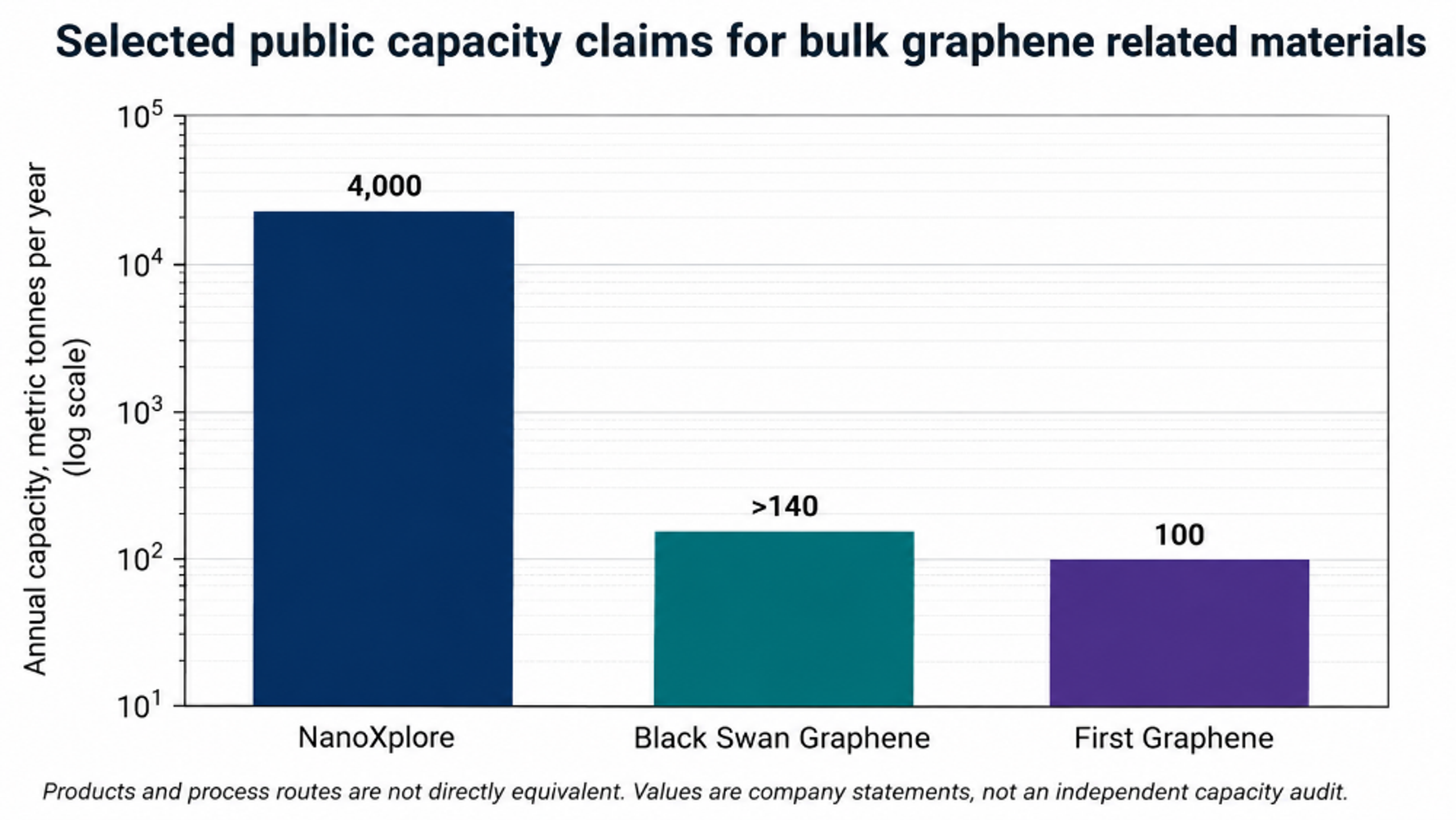
Commercial graphene related products are manufactured by several routes, many of which are not fully disclosed. Cavitation processes therefore compete with shear exfoliation, electrochemical routes, plasma expansion, chemical oxidation, thermal expansion, and proprietary combinations. Public capacity statements are useful manufacturing benchmarks, but products with different layer counts, purity, lateral size, and formulation cannot be compared by tonnage alone.
Figure 15.1. Selected publicly stated annual capacities for graphene related materials. NanoXplore reports 4,000 t y⁻¹, Black Swan Graphene reports more than 140 t y⁻¹ after its March 2026 expansion, and First Graphene reports a 100 t y⁻¹ plant [25-27]Source citations in original document: [25-27].
*[Figure 15.1](#figure-15-1). Selected publicly stated annual capacities for graphene related materials. NanoXplore reports 4,000 t y⁻¹, Black Swan Graphene reports more than 140 t y⁻¹ after its March 2026 expansion, and First Graphene reports a 100 t y⁻¹ plant [25-27].*
NanoXplore describes GrapheneBlack powder with a predominant thickness of six to ten atomic layers, purity of 96 to 98 percent, and a fully automated facility capable of producing 4,000 metric tons per year [25]. Black Swan Graphene announced completion of a United Kingdom expansion on 18 March 2026, reporting more than 140 tons per year of graphene nanoplatelet capacity and industrial flow rates up to 22,000 L h⁻¹ [26]. First Graphene reports a 100 tons per year plant for PureGRAPH products [27]. Directa Plus describes a physical plasma super expansion route that produces pristine graphene nanoplatelets in powder, liquid, and paste forms [28]. These examples indicate that the market is oriented toward consistent, application ready bulk materials rather than monolayer graphene alone.
*Table 15.1. Selected industrial benchmarks relevant to bulk graphene materials.*
| **Organization** | **Public product or route description** | **Public scale statement** | **Relevance to cavitation development** |
|----------------------|----------------------------------------------------------------------------------------------------------------|--------------------------------------------------------------------------------------------------|----------------------------------------------------------------------------------------------|
| NanoXplore | GrapheneBlack powder and integrated composite products; proprietary mechanical liquid exfoliation description. | 4,000 metric tons per year facility; predominant 6 to 10 layers; 96 to 98% purity [25]. | Sets a high volume benchmark for cost, consistency, and downstream integration. |
| Black Swan Graphene | Graphene nanoplatelets and masterbatch products using high shear liquid processing. | More than 140 t y⁻¹ after March 2026 expansion; up to 22,000 L h⁻¹ flow [26]. | Shows industrial relevance of high pressure homogenization and continuous liquid processing. |
| First Graphene | PureGRAPH powders, dispersions, and masterbatches. | 100 t y⁻¹ manufacturing capacity [27]. | Benchmark for application specific grades, quality release, and customer integration. |
| Directa Plus | Pristine graphene nanoplatelets made by plasma super expansion and physical processing. | Modular industrial process; products supplied as powder, liquid, paste, and hybrid forms [28]. | Comparator demonstrating that cavitation must compete with other physical top down routes. |
| Microfluidics / IDEX | High pressure Microfluidizer interaction chambers and application support. | Supplier states scale from laboratory units to hundreds of liters per hour [20]. | Commercial equipment platform for concentrated, repeatable high shear processing. |
## 16 Environmental Health, Safety, and Responsible Manufacturing
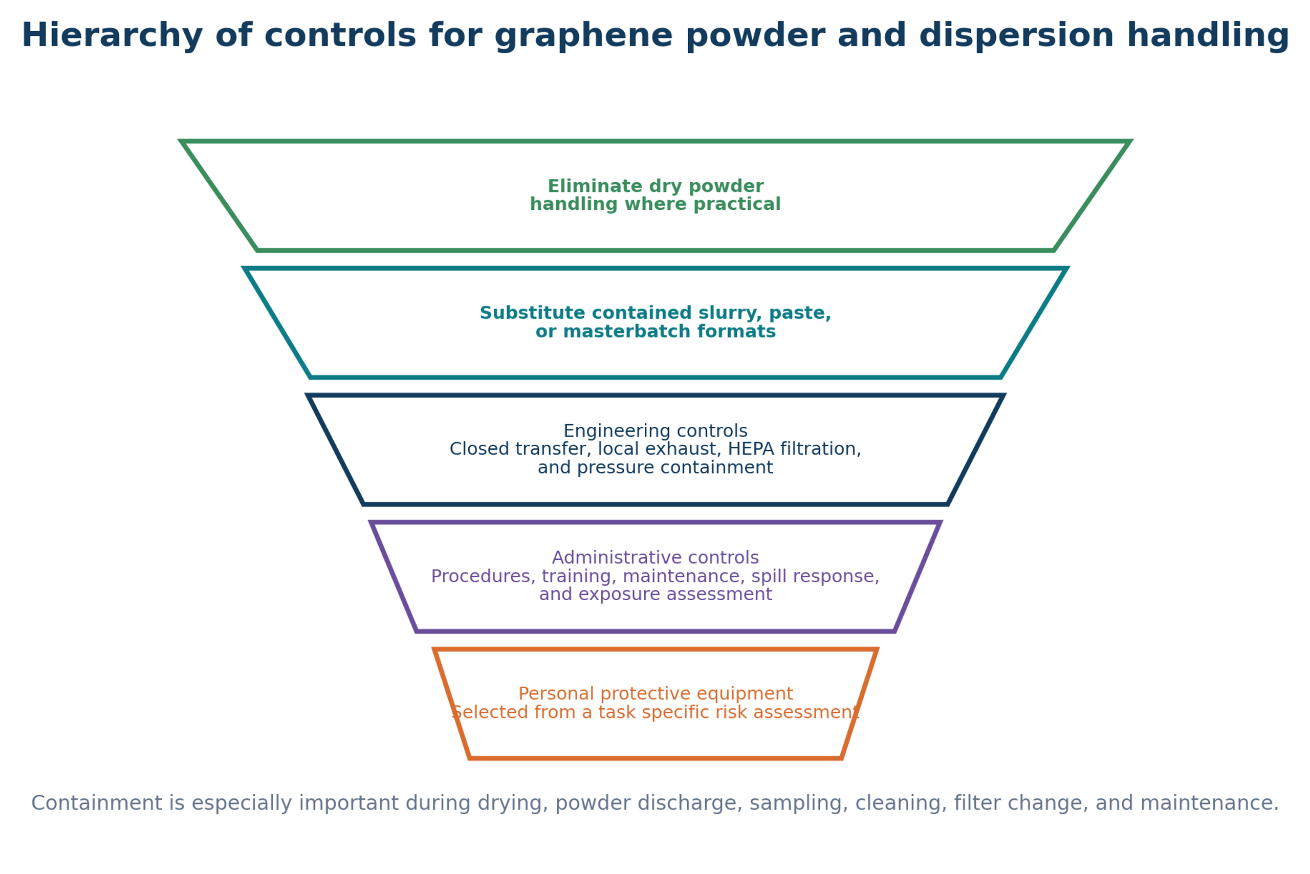
Graphene related nanomaterials can become airborne during drying, powder discharge, bag opening, blending, sampling, maintenance, filter replacement, and cleanup. Toxicology and exposure information continues to develop, and broadly accepted occupational exposure limits are not established for all graphene forms. A practical approach is prevention through design, containment, exposure assessment, and a hierarchy of controls. ISO/TS 12901-1:2024 addresses occupational risk management for materials that contain and release nano objects, while ISO/TS 12901-2:2026 provides a control banding approach when quantitative toxicology and exposure data are limited [29,30].
Figure 16.1. Hierarchy of controls for graphene powder and dispersion handling. Contained liquid, paste, or masterbatch formats can reduce free powder exposure [37]Source citation in original document: [37].
*[Figure 16.1](#figure-16-1). Hierarchy of controls for graphene powder and dispersion handling. Contained liquid, paste, or masterbatch formats can reduce free powder exposure [37].*
OSHA guidance recommends minimizing worker exposure to nanomaterials and avoiding open air handling of free particles when practical. Closed containers, local exhaust ventilation, HEPA filtered capture, appropriate cleaning methods, and task specific personal protective equipment are core controls [31,32]. Pressurized systems additionally require pressure relief, interlocks, guards, compatible fittings, and controlled depressurization. Organic liquids introduce fire, vapor, and solvent exposure hazards, while cavitation equipment can introduce noise and vibration. A complete process hazard analysis should evaluate these hazards together.
### 16.1 Dust and Aerosol Control
> • Prefer slurry, paste, or masterbatch transfer over dry powder transfer when product requirements allow.
>
> • Use sealed charging, contained sampling, enclosed filtration, and local exhaust at unavoidable release points.
>
> • Do not use dry sweeping or compressed air for cleanup. Use HEPA filtered vacuum methods or wet cleaning compatible with the material and facility.
>
> • Monitor both background and task based aerosol concentrations using a tiered strategy that distinguishes incidental particles from process material.
>
> • Treat used filters, wipes, protective clothing, and spill residues as nanomaterial contaminated waste according to the site waste plan.
### 16.2 Solvent, Pressure, and Mechanical Safety
> • Select pump, valve, hose, seal, and vessel ratings above the maximum credible pressure, including blocked outlet and thermal expansion cases.
>
> • Provide engineered pressure relief and verify safe discharge location. Do not rely only on software limits.
>
> • Interlock access to moving rotors, intensifier pumps, and pressurized interaction chambers.
>
> • Control solvent vapor through closed recovery, ventilation, bonding and grounding, and ignition source management.
>
> • Measure noise and vibration around cavitating jets and ultrasonic equipment; apply isolation and hearing protection where required.
### 16.3 Environmental Accounting
A water based process is not automatically environmentally preferable if it uses very dilute solids, prolonged recirculation, high cooling duty, energy intensive centrifugation, and disposable filters. Conversely, an organic process is not automatically unacceptable if the solvent is efficiently recovered in a closed loop. Environmental comparison should include raw graphite, stabilizer, solvent makeup, electricity, cooling water, filter media, cleaning liquid, reject solids, emissions, and final product performance. The functional unit should be one kilogram of in specification material or one unit of application performance, not one liter of treated suspension.
## 17 Critical Comparison and Conclusions
Acoustic cavitation remains valuable because it is flexible, accessible, and well suited to screening frequency, amplitude, pressure, pulse mode, liquid composition, and mechanism. Its principal limitation is field nonuniformity during direct batch scale up. Hydrodynamic cavitation is more naturally compatible with continuous operation because pressure drop, flow, geometry, back pressure, and pass count can be defined. Its principal limitations are wear, pressure containment, blockage, heat removal, and flake fragmentation. Microfluidization and wet jet milling provide high shear and high throughput at the cost of capital intensity and possible flake cutting. Rotor stator processing is widely available and useful for premixing and moderate exfoliation, although its active mechanisms are more difficult to isolate.
Figure 17.1. Conceptual tradeoff among exfoliation yield, lateral size retention, defect formation, and process burden as cavitation severity increases [37]Source citation in original document: [37].
*[Figure 17.1](#figure-17-1). Conceptual tradeoff among exfoliation yield, lateral size retention, defect formation, and process burden as cavitation severity increases [37].*
The combined literature shows that treatment severity has an optimum. Increasing time, pressure, cycle count, or acoustic power can produce thinner material, but it can also reduce lateral size, increase edge density, produce holes, degrade stabilizers, increase contamination, and lower isolated yield. The optimum is application specific. Conductive inks may benefit from small stable flakes, whereas structural composites may require platelets with high aspect ratio. A catalyst support may benefit from increased edge density, while an electronic film may reject the same defect population.
Industrial performance depends on the complete process line. Feed qualification, wetting, cavitation or high shear treatment, cooling, classification, solvent recovery, drying or formulation, quality assurance, cleaning, safety, and application conversion must be designed as one integrated system. Reactor yield before separation is not a sufficient commercial metric. A more defensible metric is the reproducible mass of in specification material produced per unit time, energy, cost, and environmental burden.
For many high volume applications, a consistent few layer graphene or graphene nanoplatelet product is more valuable than a small monolayer fraction embedded within a broad distribution. Development should therefore be specification driven. Cavitation is a powerful process intensification tool within that strategy when pressure history, residence time, chemistry, product classification, and downstream consequences are measured and controlled.
## Nomenclature
Symbols are listed in the order used in this article. Unless otherwise stated, quantities are expressed in SI units.
| **Symbol** | **Meaning** | **Unit** |
|---------------------|----------------------------------------------------------------------------------------------------------------|---------------------|
| A | Projected flake area, newly created surface area, or optical absorbance when written as Aλ; context is stated. | m² or dimensionless |
| | Absorbance at wavelength λ. | dimensionless |
| | Equivalent flake aspect ratio. | dimensionless |
| Atr | Active transducer area. | m² |
| C | Dispersed nanosheet concentration. | kg m⁻³ or g L⁻¹ |
| | Initial dispersed concentration. | kg m⁻³ or g L⁻¹ |
| cp | Specific heat capacity. | J kg⁻¹ K⁻¹ |
| deq | Equivalent particle diameter used in a sedimentation approximation. | m |
| d95 | Particle size below which 95 percent of the feed distribution falls. | m |
| Dh | Hydraulic diameter. | m |
| | Specific process energy per mass of recovered product. | J kg⁻¹ |
| ER | Erosion rate is based on mass loss. | kg m⁻² s⁻¹ |
| Esys | Total energy within the selected process boundary. | J |
| Eu | Euler type pressure coefficient. | dimensionless |
| Ev | Cumulative hydraulic energy density. | J m⁻³ |
| g | Gravitational acceleration, or effective gap when identified in a shear rate relation. | m s⁻² or m |
| Gc | Effective cleavage energy per unit area. | J m⁻² |
| h | Nanosheet thickness. | m or nm |
| | Calibrated apparent AFM thickness per layer. | m or nm |
| | Irreversible head loss. | m |
| Iac | Nominal acoustic intensity. | W m⁻² |
| ID, IG, I2D | Raman intensities of D, G, and 2D bands. | arbitrary units |
| La | Empirical in plane crystallite or defect spacing estimate. | nm |
| l | Optical path length. | m |
| m | Liquid mass in calorimetry. | kg |
| | Dry starting mass of layered solid. | kg |
| | Coarse reject or recycle mass. | kg |
| | Fine fraction mass. | kg |
| | Unaccounted mass loss. | kg |
| | Recovered product mass. | kg |
| | Recovered mass meeting the complete product specification. | kg |
| N | Approximate number of layers. | dimensionless |
| Np | Number of process passes or cycles. | dimensionless |
| n | Centrifuge rotational speed. | min⁻¹ |
| p | Static pressure. | Pa |
| | Pressure inside a bubble. | Pa |
| | Far field liquid pressure. | Pa |
| | Reference upstream pressure. | Pa |
| | Liquid vapor pressure. | Pa |
| Pac | Acoustic power delivered to the liquid. | W |
| Pcal | Calorimetrically measured acoustic power. | W |
| Ph | Hydraulic pump power is associated with the useful pressure drop. | W |
| Q | Volumetric flow rate. | m³ s⁻¹ |
| R | Bubble radius. | m |
| RCF | Relative centrifugal force. | multiples of g |
| Re | Reynolds number. | dimensionless |
| Rp | Usable production rate. | kg s⁻¹ or kg h⁻¹ |
| S(t) | Normalized dispersion stability index. | dimensionless |
| t | Time. | s |
| tc | Idealized bubble collapse time. | s |
| texp | Cumulative nominal exposure time. | s |
| u | Characteristic liquid velocity. | m s⁻¹ |
| | Terminal settling velocity in a Stokes approximation. | m s⁻¹ |
| Vactive | Active reactor volume. | m³ |
| Wmin | Ideal minimum work to create new surfaces. | J |
| Yusable | Usable product yield. | % |
| z | Elevation head coordinate. | m |
### Greek Letters
| **Symbol** | **Meaning** | **Unit** |
|------------|---------------------------------------------------------|----------------------|
| αλ | Optical extinction coefficient at wavelength λ. | m² kg⁻¹ or L g⁻¹ m⁻¹ |
| γ | Liquid surface tension. | N m⁻¹ |
| γ̇ | Shear rate. | s⁻¹ |
| δD | Dispersive Hansen solubility parameter component. | MPa¹ᐟ² |
| δP | Polar Hansen solubility parameter component. | MPa¹ᐟ² |
| δH | Hydrogen bonding Hansen solubility parameter component. | MPa¹ᐟ² |
| Δp | Pressure difference across the active element. | Pa |
| Δρ | Density difference between particle and liquid. | kg m⁻³ |
| Δu | Velocity difference across a gap or boundary layer. | m s⁻¹ |
| ηE | Mass based energy efficiency. | kg J⁻¹ |
| ηp | Overall pump efficiency. | dimensionless |
| κ | Selected conservative blockage ratio. | dimensionless |
| λ | Optical wavelength. | m or nm |
| λL | Raman laser wavelength. | nm |
| μ | Dynamic viscosity. | Pa s |
| ρ | Liquid density. | kg m⁻³ |
| σ | Cavitation number. | dimensionless |
| τ | Viscous shear stress. | Pa |
| τpass | Nominal residence time in the active region per pass. | s |
## Abbreviations
| **Abbreviation** | **Meaning** |
|------------------|--------------------------------------------------|
| AFM | Atomic force microscopy |
| BSA | Bovine serum albumin |
| CMC | Carboxymethyl cellulose |
| DLS | Dynamic light scattering |
| FTIR | Fourier transform infrared spectroscopy |
| GNP | Graphene nanoplatelet |
| GR2M | Graphene related two dimensional material |
| hBN | Hexagonal boron nitride |
| HC | Hydrodynamic cavitation |
| HRTEM | High resolution transmission electron microscopy |
| ICP MS | Inductively coupled plasma mass spectrometry |
| LPE | Liquid phase exfoliation |
| LOC | Lab on a chip |
| MoS₂ | Molybdenum disulfide |
| PVP | Polyvinylpyrrolidone |
| SEM | Scanning electron microscopy |
| TEM | Transmission electron microscopy |
| TGA | Thermogravimetric analysis |
| UV Vis | Ultraviolet visible spectroscopy |
| WJM | Wet jet milling |
| WS₂ | Tungsten disulfide |
| XPS | X ray photoelectron spectroscopy |
| XRD | X ray diffraction |
## Bibliography
[1] K. S. Novoselov, A. K. Geim, S. V. Morozov, D. Jiang, Y. Zhang, S. V. Dubonos, I. V. Grigorieva, and A. A. Firsov, Electric field effect in atomically thin carbon films, Science, 306(5696), 666-669, 2004. doi:10.1126/science.1102896.
[2] A. C. Ferrari, J. C. Meyer, V. Scardaci, C. Casiraghi, M. Lazzeri, F. Mauri, S. Piscanec, D. Jiang, K. S. Novoselov, S. Roth, and A. K. Geim, Raman spectrum of graphene and graphene layers, Physical Review Letters, 97, 187401, 2006. doi:10.1103/PhysRevLett.97.187401.
[3] International Organization for Standardization, ISO/TS 80004-13:2024, Nanotechnologies, Vocabulary, Part 13: Graphene and other two dimensional materials, Geneva, 2024.
[4] International Organization for Standardization, ISO/TS 21356-1:2021, Nanotechnologies, Structural characterization of graphene, Part 1: Graphene from powders and dispersions, Geneva, 2021.
[5] International Organization for Standardization, ISO/TS 23359:2025, Nanotechnologies, Chemical characterization of graphene related two dimensional materials from powders and liquid dispersions, Geneva, 2025.
[6] International Organization for Standardization, ISO/TS 9651:2025, Nanotechnologies, Classification framework for graphene related two dimensional materials, Geneva, 2025.
[7] Z. Shen, J. Li, M. Yi, X. Zhang, and S. Ma, Preparation of graphene by jet cavitation, Nanotechnology, 22, 365306, 2011. doi:10.1088/0957-4484/22/36/365306.
[8] M. Yi, J. Li, Z. Shen, X. Zhang, and S. Ma, Morphology and structure of mono and few layer graphene produced by jet cavitation, Applied Physics Letters, 99, 123112, 2011. doi:10.1063/1.3641863.
[9] S. Liang, Z. Shen, M. Yi, L. Liu, X. Zhang, C. Cai, and S. Ma, Effects of processing parameters on massive production of graphene by jet cavitation, Journal of Nanoscience and Nanotechnology, 15, 2686-2694, 2015. doi:10.1166/jnn.2015.9201.
[10] X. Qiu, V. Bouchiat, D. Colombet, and F. Ayela, Liquid phase exfoliation of graphite into graphene nanosheets in a hydrocavitating lab on a chip, RSC Advances, 9, 3232-3238, 2019. doi:10.1039/C8RA05976D. Licensed CC BY NC 3.0.
[11] M. Jafarpour, A. S. Aghdam, M. T. Gevari, A. Koşar, M. K. Bayazıt, and M. Ghorbani, An ecologically friendly process for graphene exfoliation based on the hydrodynamic cavitation on a chip concept, RSC Advances, 11, 17965-17975, 2021. doi:10.1039/D1RA03352B. Licensed CC BY 3.0.
[12] S. De Alwis, M. A. Shirsavar, S. Singh, and N. N. Hashemi, Hydrodynamic cavitation for scalable exfoliation of few layered graphene nanosheets, Nanotechnology, 32, 505701, 2021. doi:10.1088/1361-6528/ac2096.
[13] C. H. Choi, Y. Kwak, R. Malhotra, and C. H. Chang, Microfluidics for two dimensional nanosheets: A mini review, Processes, 8, 1067, 2020. doi:10.3390/pr8091067. Licensed CC BY 4.0.
[14] O. P. Stebeleva, L. V. Kashkina, O. A. Vshivkova, and A. V. Minakov, Application of high speed hydrodynamic technology for the production of graphene nanosuspensions from natural graphite’s, Siberian Aerospace Journal, 25(4), 521-530, 2024. doi:10.31772/2712-8970-2024-25-4-521-530.
[15] L. Liu, Z. Shen, M. Yi, X. Zhang, and S. Ma, A green, rapid and size controlled production of high quality graphene sheets by hydrodynamic forces, RSC Advances, 4, 36464-36470, 2014. doi:10.1039/C4RA05635C.
[16] N. Liu, Q. Tang, B. Huang, and Y. Wang, Graphene synthesis: Method, exfoliation mechanism and large scale production, Crystals, 12, 25, 2022. doi:10.3390/cryst12010025. Licensed CC BY 4.0.
[17] K. Xiang et al., Ultrasonic cavitation shock wave exfoliation dynamics of two dimensional materials revealed in situ by MHz XFEL imaging and multiphysics modeling, Science Advances, 11(48), eady9558, 2025. doi:10.1126/sciadv.ady9558.
[18] W. Qiao, S. Yan, X. He, X. Song, Z. Li, X. Zhang, W. Zhong, and Y. Du, Effects of ultrasonic cavitation intensity on the efficient liquid exfoliation of MoS₂ nanosheets, RSC Advances, 4, 50981-50987, 2014. doi:10.1039/C4RA09001B.
[19] D. T. Nguyen, H. A. Ting, Y. H. Su, M. Hofmann, and Y. P. Hsieh, Additive enhanced exfoliation for high yield two dimensional materials production, Nanomaterials, 11, 601, 2021. doi:10.3390/nano11030601. Licensed CC BY 4.0.
[20] Microfluidics International Corporation, Use of Microfluidizer technology for graphene exfoliation, application note and conductive ink case study, Westwood, Massachusetts, accessed August 5, 2026.
[21] P. G. Karagiannidis et al., Microfluidization of graphite and formulation of graphene based conductive inks, ACS Nano, 11(3), 2742-2755, 2017. doi:10.1021/acsnano.6b07735.
[22] B. Z. Jang, A. Zhamu, and J. Guo, Production of graphene materials in a cavitating fluid, U.S. Patent 9,315,388 B2, April 19, 2016; corresponding publication U.S. 2015/0239741 A1.
[23] O. Kozyuk and P. Reimers, Method of forming graphene material by graphite exfoliation, U.S. Patent 9,845,244 B2, December 19, 2017.
[24] W. Yan, M. Vijay, A. Tieu, M. Xu, and B. Daniels, Apparatus and method for preparing graphene by exfoliation of graphite using a pulsed or cavitating waterjet, U.S. Patent Application 2018/0009667 A1, January 11, 2018.
[25] NanoXplore Inc., GrapheneBlack product and manufacturing information, including 4,000 metric tons per year facility and 6 to 10 layer product description, official company materials.
[26] Black Swan Graphene Inc., Black Swan Graphene completes production capacity expansion at its United Kingdom facility, official press release, March 18, 2026.
[27] First Graphene Ltd., PureGRAPH products and manufacturing capacity information, official company materials.
[28] Directa Plus plc, Annual Report and Accounts 2024 and official process information for plasma super expansion graphene nanoplatelets, 2025.
[29] International Organization for Standardization, ISO/TS 12901-1:2024, Nanotechnologies, Occupational risk management applied to engineered nanomaterials, Part 1: Principles and approaches, Geneva, 2024.
[30] International Organization for Standardization, ISO/TS 12901-2:2026, Nanotechnologies, Occupational risk management applied to engineered nanomaterials, Part 2: Use of the control banding approach, Geneva, 2026.
[31] Occupational Safety and Health Administration, Working safely with nanomaterials, OSHA Fact Sheet 3634, U.S. Department of Labor, 2013.
[32] L. M. Lo, D. Hammond, I. Bartholomew, D. Almaguer, W. Heitbrink, and J. Topmiller, Engineering controls for nano scale graphene platelets during manufacturing and handling processes, EPHB Report No. 356-12a, National Institute for Occupational Safety and Health, December 2011.
[33] E. Varrla, K. R. Paton, C. Backes, A. Harvey, R. J. Smith, J. McCauley, and J. N. Coleman, Turbulence assisted shear exfoliation of graphene using household detergent and a kitchen blender, Nanoscale, 6, 11810-11819, 2014. doi:10.1039/C4NR03560G.
[34] M. Lotya et al., Liquid phase production of graphene by exfoliation of graphite in surfactant water solutions, Journal of the American Chemical Society, 131, 3611-3620, 2009. doi:10.1021/ja807449u.
[35] A. Ciesielski and P. Samorì, Graphene via sonication assisted liquid phase exfoliation, Chemical Society Reviews, 43, 381-398, 2014. doi:10.1039/C3CS60217F.
[36] C. Backes et al., Production and processing of graphene and related materials, 2D Materials, 7, 022001, 2020. doi:10.1088/2053-1583/ab1e0a.
[37] Kozyuk O. Hydrodynamic Cavitation. [Unpublished technical manuscript and supporting data] 2026.